Bonjour Habr! Par ma profession principale, je suis ingénieur pour le développement des champs pétroliers et gaziers. Je viens de plonger dans Data Sciense et c'est mon premier article pour partager mon expérience de l'apprentissage automatique dans l'industrie pétrolière.

. , , .
. , ( ).
, . .
:
( + ) () () , .
( ). () . , , - - , .
, , . .
3D ().
, ( ). . , . . . . 10 - 15 . , 3- 250 - 1000 . , , " ".
. . . - , . - 3- ( , ) ( ). . , .
. .
:
( , , /- , , ..),
- , , .
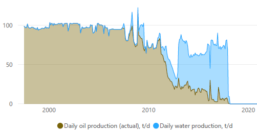
. . , . , . , - . .. Q/(Q + Q)*100%
( ) :
:
Cum oil:
Days: ( ( ) ).
In prod: /
Q oil:
wct:
Top perf: -
Bottom perf:
ST: 0 - , 1 -
x, y:
import numpy as np
import pandas as pd
import matplotlib.pyplot as plt
%matplotlib inline
%config InlineBackend.figure_format = 'svg'
import pylab
from pylab import rcParams
import plotly.express as px
import plotly.graph_objects as go
from sklearn.model_selection import train_test_split
from sklearn.ensemble import RandomForestRegressor
from sklearn.metrics import r2_score as r2, mean_absolute_error as mae, mean_squared_error as mse, accuracy_score
from sklearn.metrics.pairwise import euclidean_distances
.
data_path = 'art_df.xlsx'
df = pd.read_excel(data_path, sheet_name='artificial')
df

- . ( ).
ax = df.plot(kind='scatter', x='x', y='y')
df[['x','y','Well']].apply(lambda row: ax.text(*row),axis=1);
rcParams['figure.figsize'] = [11, 8]
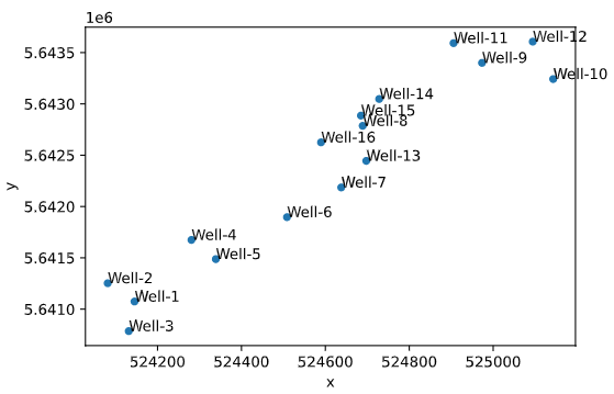
, " " . . , , .
.
distance = pd.DataFrame(euclidean_distances(df[['x', 'y']]))
distance
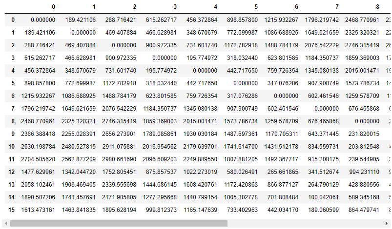
. .
well_names = df['Well']
distance.columns = well_names
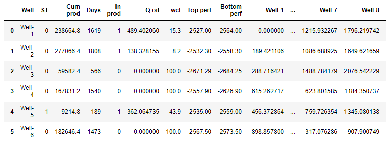
. - , .
df_distance = pd.concat([df.drop(['x', 'y'], axis=1), distance], axis=1)
df_distance
. , ,
df_train_1 = df_distance.drop([12, 13, 14, 15], axis=0)
df_train_1

df_test_1 = df_distance.loc[[12, 13]]
df_test_1

DataFrame X_1. ( ) wct.
x_1 = df_train_1.drop(['Well', 'wct'], axis=1)
x_1

y_1
y_1 = df_train_1['wct']
y_test_1
y_test_1 = df_test_1['wct']
Random Forest Reggressor, , .
x_test_1 = df_test_1.drop(['Well', 'wct'], axis=1)
model = RandomForestRegressor(random_state=42, max_depth=14)
model.fit(x_1, y_1)
y_pred_train_1 = model.predict(x_1)
y_pred_1 = model.predict(x_test_1)
print('Predicted values from train data:')
r2_train = r2(y_1, y_pred_train_1)
mae_train = mae(y_1, y_pred_train_1)
mse_train = mse(y_1, y_pred_train_1)
print(f'R2 train: {r2_train.round(4)}')
print(f'MAE train: {mae_train.round(4)}')
print(f'MSE train: {mse_train.round(4)}')
print('Predicted values from test data:')
r2_test = r2(y_test_1, y_pred_1)
mae_test = mae(y_test_1, y_pred_1)
mse_test = mse(y_test_1, y_pred_1)
print(f'R2 test: {r2_test.round(4)}')
print(f'MAE test: {mae_test.round(4)}')
print(f'MSE test: {mse_test.round(4)}')
model
Predicted values from train data:
R2 train: 0.8832
MAE train: 8.2855
MSE train: 131.1208
Predicted values from test data:
R2 test: 0.8758
MAE test: 3.164
MSE test: 11.4485
RandomForestRegressor(max_depth=14, random_state=42)
R2 R2 1%. , .
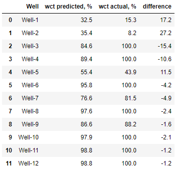
, (blind test)
df_y_test = pd.DataFrame({'Well': df_test_1['Well'],
'wct predicted, %': y_pred_1.round(1),
'wct actual, %': y_test_1.round(1),
'difference': (y_pred_1 - y_test_1).round(1)})
df_y_test

df_y_train = pd.DataFrame({'Well': df_train_1['Well'],
'wct predicted, %': y_pred_train_1.round(1),
'wct actual, %': y_1.round(1),
'difference': (y_pred_train_1 - y_1).round(1)})
df_y_train
:
round(sum(abs(y_pred_train_1 - y_1)) / len(y_1), 1)
8.3
, 8%, .
, ,
df_train_2 = df_distance.drop([14, 15], axis=0)
, .
WCT () = NaN.
df_fc = df_distance.loc[[14, 15]]
DataFrame x_2. ( ) wct.
x_2 = df_train_2.drop(['Well', 'wct'], axis=1)
y_2 .
y_2 = df_train_2['wct']
x_fc = df_fc.drop(['Well', 'wct'], axis=1)
model = RandomForestRegressor(random_state=42, max_depth=14)
model.fit(x_2, y_2)
y_pred_train_2 = model.predict(x_2)
y_fc = model.predict(x_fc)
print('Predicted values from train data:')
r2_train = r2(y_2, y_pred_train_2)
mae_train = mae(y_2, y_pred_train_2)
mse_train = mse(y_2, y_pred_train_2)
print(f'R2 train: {r2_train.round(4)}')
print(f'MAE train: {mae_train.round(4)}')
print(f'MSE train: {mse_train.round(4)}')
print('Forecasted values could be compared with real data!')
model
Predicted values from train data:
R2 train: 0.9095
MAE train: 6.5196
MSE train: 89.9625
RandomForestRegressor(max_depth=14, random_state=42)
R2 .
.
df_y_train = pd.DataFrame({'Well': df_train_2['Well'],
'wct predicted, %': y_pred_train_2.round(1),
'wct actual, %': y_2.round(1),
'difference': (y_pred_train_2 - y_2).round(1)})
df_y_train
round(sum(abs(y_pred_train_2 - y_2)) / len(y_2), 1)
6,5
6,5. !
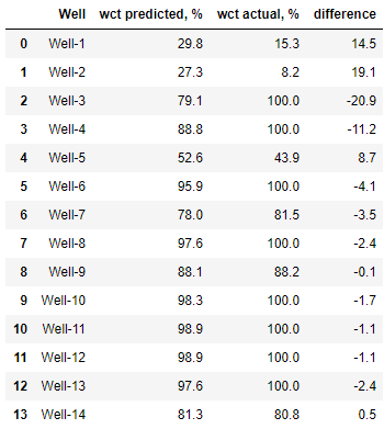
:
df_y_test = pd.DataFrame({'Well': df_test_1['Well'],
'wct predicted, %': y_pred_1.round(1),
'wct actual, %': y_test_1.round(1),
'difference': (y_pred_1 - y_test_1).round(1)})
df_y_test

.
model.feature_importances_
feature_importances = pd.DataFrame()
feature_importances['feature_name'] = x_2.columns.tolist()
feature_importances['importance'] = model.feature_importances_
feature_importances = feature_importances.sort_values(by='importance', ascending=False)
feature_importances
fig = px.bar(feature_importances,
x=feature_importances['importance'],
y=feature_importances['feature_name'],
title="Feature importances")
fig.update_layout(yaxis={'categoryorder':'total ascending'})
fig.show()
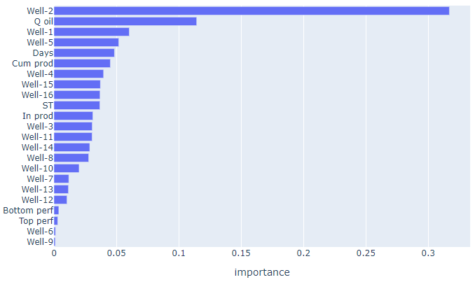
, - 2- . .
. - .
fig = px.scatter(x=y_pred_train_2, y=y_2, title="True vs Predicted values",
text=df_train_2['Well'], width=850, height=800)
fig.add_trace(go.Scatter(x=[0,100], y=[0,100], mode='lines', name='True=Predicted',
line = dict(color='red', width=1, dash='dash')))
fig.update_xaxes(title_text='Predicted')
fig.update_yaxes(title_text='True')
fig.show()

. (- ), (, ).
, " " . , , .
. - "" - .

. " ", . "" . . , .
, . , .
Les données de puits ne sont pas des données ouvertes, mais sont la propriété de la société détentrice de la licence pour développer le domaine. Par conséquent, pour illustrer le travail effectué, des données de puits artificiels ont été générées qui sont disponibles pour ce travail.
Le code source ainsi que le texte de l'article sont disponibles ici: https://github.com/alex-kalinichenko/re/tree/master/wct_fc