Introduction: Concurrence du groupe financier HOME CREDIT pour déterminer le risque de défaut de l'emprunteur

Cet article traite du concours d'apprentissage automatique du  risque de défaut de crédit immobilier, qui vise à utiliser des données historiques sur les demandes de prêt pour prédire si un demandeur sera en mesure de rembourser un prêt (déterminer le risque de défaut d'un emprunteur). Prédire si un client remboursera un prêt ou rencontrera des problèmes est un défi commercial critique, et Home Credit organise un concours sur la plate-forme Kaggle pour voir quels modèles d'apprentissage automatique la communauté peut développer pour les aider à relever ce défi.

Il s'agit d'une tâche de classification supervisée standard:

• Apprentissage supervisé: les réponses correctes sont incluses dans les données de formation et le but est de former le modèle à prédire ces réponses en fonction des indices disponibles.

  
  
  
  
  

• : , – 0 ( ) 1 ( ).

  
  
  
  
  

Home Credit, () , . 7 :

• applicationtrain / applicationtest: Home Credit. ,  SKIDCURR  .  TARGET  :

  
  
  
  
  

  • 0, ;

    
    
    
    
    

  • 1, .

    
    
    
    
    

• bureau: . , .

  
  
  
  
  

• bureaubalance: . . , .

  
  
  
  
  

• previousapplication: Home Credit , . ,  SKIDPREV.

  
  
  
  
  

• POSCASHBALANCE: , Home Credit. , .

  
  
  
  
  

• creditcardbalance: , Home Credit. . .

  
  
  
  
  

• installments_payment: Home Credit, .

  
  
  
  
  

, :

, (  HomeCredit_columns_description.csv) .

(application_train / application_test), . , . , ! - , .

: ROC AUC

( ), , . ,  (ROC AUC, AUROC).

ROC AUC , , .

(ROC)  , , , , :

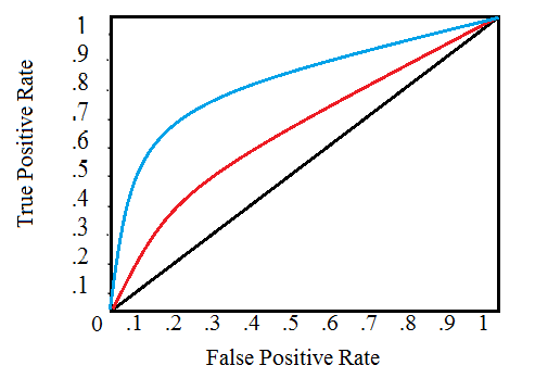
, , . 0 1 . , , . , , , , , , ( ).

(AUC)  . ROC ( ). 0 1, . , , ROC AUC = 0,5.

ROC AUC, 0 1, 0 1. , , , ( , ) — . , , 99,9999%, , , . , ( ), , ROC AUC F1, . ROC AUC , ROC AUC .

, , . , , . .

: numpy  pandas  , sklearn preprocessing  , matplotlib ¨C11C¨C12C¨C13C . .

import os
import numpy as np
import pandas as pd
pd.set_option('display.max_columns', None)
from sklearn.preprocessing import LabelEncoder
import matplotlib.pyplot as plt
import seaborn as sns

#  
import warnings
warnings.filterwarnings('ignore')
      
      

        
        
        
      

    
        
        
        
      
      

        
        
        
      

    
    

, , . 9 : ( ), ( ), 6 , .

#   
print(os.listdir("../input/"))
      
      

        
        
        
      

    
        
        
        
      
      

        
        
        
      

    
    

‘POSCASHbalance.csv’, ‘bureaubalance.csv’, ‘applicationtrain.csv’, ‘previousapplication.csv’, ‘installmentspayments.csv’, ‘creditcardbalance.csv’, ‘samplesubmission.csv’, ‘applicationtest.csv’, ‘bureau.csv’]

#  
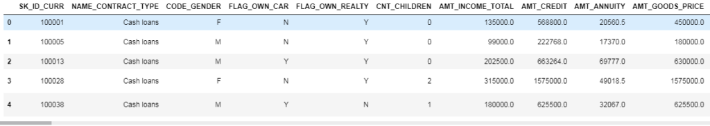
app_train = pd.read_csv('../input/application_train.csv')
print('Training data shape: ', app_train.shape)
app_train.head()
      
      

        
        
        
      

    
        
        
        
      
      

        
        
        
      

    
    

Training data shape: (307511, 122)

307511 , 120 , , .

#  
app_test = pd.read_csv('../input/application_test.csv')
print('Testing data shape: ', app_test.shape)
app_test.head()
      
      

        
        
        
      

    
        
        
        
      
      

        
        
        
      

    
    

Testing data shape: (48744, 121)

, TARGET.

(EXPLORATORY DATA ANALYSIS – EDA)

(EDA) — , , , , . EDA — , . , , . , , , , .

— , : 0, , 1, . , .

app_train['TARGET'].value_counts()
      
      

        
        
        
      

    
        
        
        
      
      

        
        
        
      

    
    

app_train['TARGET'].astype(int).plot.hist();
      
      

        
        
        
      

    
        
        
        
      
      

        
        
        
      

    
    

, . , , , . ,     , .

.

#        
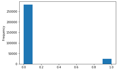
def missing_values_table(df):
        #    
        mis_val = df.isnull().sum()
        #   
        mis_val_percent = 100 * df.isnull().sum() / len(df)
        #    
        mis_val_table = pd.concat([mis_val, mis_val_percent], axis=1)
        #  
        mis_val_table_ren_columns = mis_val_table.rename(
        columns = {0 : 'Missing Values', 1 : '% of Total Values'})
        #          
        mis_val_table_ren_columns = mis_val_table_ren_columns[
            mis_val_table_ren_columns.iloc[:,1] != 0].sort_values(
        '% of Total Values', ascending=False).round(1)
        #   
        print("Your selected dataframe has " + str(df.shape[1]) + " columns.\n"      
            "There are " + str(mis_val_table_ren_columns.shape[0]) +
              " columns that have missing values.")
        return mis_val_table_ren_columns

#   
missing_values = missing_values_table(app_train)
missing_values.head(10)
      
      

        
        
        
      

    
        
        
        
      
      

        
        
        
      

    
    

Your selected dataframe has 122 columns.

There are 67 columns that have missing values.

, - . , XGBoost,   . – , , . .

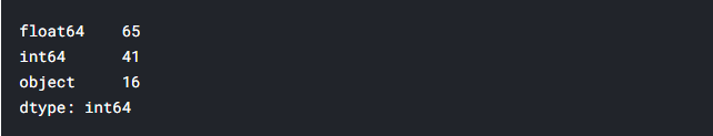
. int64  float64 — ( ).  object    .

#     
app_train.dtypes.value_counts()
      
      

        
        
        
      

    
        
        
        
      
      

        
        
        
      

    
    

 object().

#        
app_train.select_dtypes('object').apply(pd.Series.nunique, axis = 0)
      
      

        
        
        
      

    
        
        
        
      
      

        
        
        
      

    
    

, . .

, . , ( ,  LightGBM). , () , . :

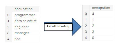
(Label encoding): . . :

(One-hot encoding): . 1 0 .

, . , , - . 4, — 1, , . . , , (, = 4 = 1) , , . (, / ), , .

, , . – Kaggle-master Will Koehrsen, , , . . , ( ) - . ,  PCA    , ( , ).

Label Encoding 2 One-Hot Encoding 2 . , , , , . - .

Label Encoding One-Hot Encoding

: (dtype == object) , – .

LabelEncoder Scikit-Learn, – pandas get_dummies(df).

#   label encoder
le = LabelEncoder()
le_count = 0
#    
for col in app_train:
    if app_train[col].dtype == 'object':
        #    2    
        if len(list(app_train[col].unique())) <= 2:
            #  LabelEncoder   
            le.fit(app_train[col])
            #     
            app_train[col] = le.transform(app_train[col])
            app_test[col] = le.transform(app_test[col])
            
            # ,     LabelEncoder
            le_count += 1
print('%d columns were label encoded.' % le_count)
      
      

        
        
        
      

    
        
        
        
      
      

        
        
        
      

    
    

3 columns were label encoded.

#  one-hot encoding   
app_train = pd.get_dummies(app_train)
app_test = pd.get_dummies(app_test)
print('Training Features shape: ', app_train.shape)
print('Testing Features shape: ', app_test.shape)
      
      

        
        
        
      

    
        
        
        
      
      

        
        
        
      

    
    

raining Features shape: (307511, 243)

Testing Features shape: (48744, 239).

(). , , . . ( , ). , axis = 1, , !

train_labels = app_train['TARGET']
#     ,   ,    
app_train, app_test = app_train.align(app_test, join = 'inner', axis = 1)
#     
app_train['TARGET'] = train_labels
print('Training Features shape: ', app_train.shape)
print('Testing Features shape: ', app_test.shape)
      
      

        
        
        
      

    
        
        
        
      
      

        
        
        
      

    
    

Training Features shape:  (307511, 240)

Testing Features shape:  (48744, 239)

, . «» . - , , ( , ), .

, EDA, — . - , , .  describe. DAYS_BIRTH , . , -1 :

(app_train['DAYS_BIRTH'] / -365).describe()
      
      

        
        
        
      

    
        
        
        
      
      

        
        
        
      

    
    

— . .

app_train['DAYS_EMPLOYED'].describe()
      
      

        
        
        
      

    
        
        
        
      
      

        
        
        
      

    
    

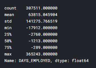
– ( , ) — 1000 !

app_train['DAYS_EMPLOYED'].plot.hist(title = 'Days Employment Histogram');
plt.xlabel('Days Employment');
      
      

        
        
        
      

    
        
        
        
      
      

        
        
        
      

    
    

, .

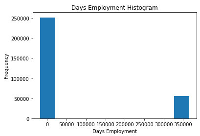
anom = app_train[app_train['DAYS_EMPLOYED'] == 365243]
non_anom = app_train[app_train['DAYS_EMPLOYED'] != 365243]
print('The non-anomalies default on %0.2f%% of loans' % (100 * non_anom['TARGET'].mean()))
print('The anomalies default on %0.2f%% of loans' % (100 * anom['TARGET'].mean()))
print('There are %d anomalous days of employment' % len(anom))
      
      

        
        
        
      

    
        
        
        
      
      

        
        
        
      

    
    

The non-anomalies default on 8.66% of loans

The anomalies default on 5.40% of loans

There are 55374 anomalous days of employment

– , .

. — , . , , , - . , , , . (np.nan), , , .

#  ,    
app_train['DAYS_EMPLOYED_ANOM'] = app_train["DAYS_EMPLOYED"] == 365243
#     nan
app_train['DAYS_EMPLOYED'].replace({365243: np.nan}, inplace = True)
app_train['DAYS_EMPLOYED'].plot.hist(title = 'Days Employment Histogram');
plt.xlabel('Days Employment');
      
      

        
        
        
      

    
        
        
        
      
      

        
        
        
      

    
    

, . , , (  nans  , , ). DAYS , , .

: , , .  np.nan  .

app_test['DAYS_EMPLOYED_ANOM'] = app_test["DAYS_EMPLOYED"] == 365243
app_test["DAYS_EMPLOYED"].replace({365243: np.nan}, inplace = True)
print('There are %d anomalies in the test data out of %d entries' % (app_test["DAYS_EMPLOYED_ANOM"].sum(), len(app_test)))
      
      

        
        
        
      

    
        
        
        
      
      

        
        
        
      

    
    

There are 9274 anomalies in the test data out of 48744 entries

, , EDA. — . ,  .corr.

— «» , .   :

• .00–0.19 « »

  
  
  
  
  

• .20-.39 «»

  
  
  
  
  

• .40–0.59 «»

  
  
  
  
  

• 0,60–0,79 «»

  
  
  
  
  

• 0,80–1,0 « »

  
  
  
  
  

#         
correlations = app_train.corr()['TARGET'].sort_values()
#   
print('Most Positive Correlations:\n', correlations.tail(15))
print('\nMost Negative Correlations:\n', correlations.head(15))
      
      

        
        
        
      

    
        
        
        
      
      

        
        
        
      

    
    

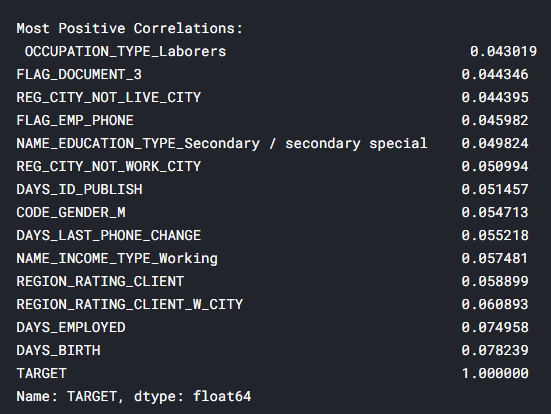
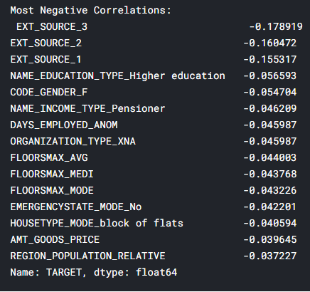
: DAYSBIRTH — ( TARGET, 1). , DAYSBIRTH — . , , , , , (.. == 0). , , .

app_train['DAYS_BIRTH'] = abs(app_train['DAYS_BIRTH'])
app_train['DAYS_BIRTH'].corr(app_train['TARGET'])
      
      

        
        
        
      

    
        
        
        
      
      

        
        
        
      

    
    

-0.07823930830982694

, , , , .

. -, . ,  x  .

plt.style.use('fivethirtyeight')
#      
plt.hist(app_train['DAYS_BIRTH'] / 365, edgecolor = 'k', bins = 25)
plt.title('Age of Client'); plt.xlabel('Age (years)'); plt.ylabel('Count');
      
      

        
        
        
      

    
        
        
        
      
      

        
        
        
      

    
    

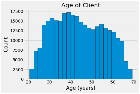
, , , . ,   (KDE), .    ( , , , ). seaborn kdeplot.

plt.figure(figsize = (10, 8))
sns.kdeplot(app_train.loc[app_train['TARGET'] == 0, 'DAYS_BIRTH'] / 365, label = 'target == 0')
sns.kdeplot(app_train.loc[app_train['TARGET'] == 1, 'DAYS_BIRTH'] / 365, label = 'target == 1')
plt.xlabel('Age (years)'); plt.ylabel('Density'); plt.title('Distribution of Ages');
      
      

        
        
        
      

    
        
        
        
      
      

        
        
        
      

    
    

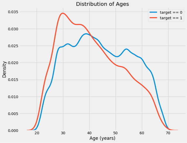
target == 1 . ( -0,07), , , , . : .

, 5 . , .

age_data = app_train[['TARGET', 'DAYS_BIRTH']]
age_data['YEARS_BIRTH'] = age_data['DAYS_BIRTH'] / 365
age_data['YEARS_BINNED'] = pd.cut(age_data['YEARS_BIRTH'], bins = np.linspace(20, 70, num = 11))
age_data.head(10)
      
      

        
        
        
      

    
        
        
        
      
      

        
        
        
      

    
    

#       
age_groups  = age_data.groupby('YEARS_BINNED').mean()
age_groups
      
      

        
        
        
      

    
        
        
        
      
      

        
        
        
      

    
    

plt.figure(figsize = (8, 8))
plt.bar(age_groups.index.astype(str), 100 * age_groups['TARGET'])
plt.xticks(rotation = 75); plt.xlabel('Age Group (years)'); plt.ylabel('Failure to Repay (%)')
plt.title('Failure to Repay by Age Group');
      
      

        
        
        
      

    
        
        
        
      
      

        
        
        
      

    
    

: . 10% 5% .

: , , . , , , .

: EXTSOURCE1, EXTSOURCE2  EXTSOURCE3. , « ». , , , , , .

.

-, EXT_SOURCE .

ext_data = app_train[['TARGET', 'EXT_SOURCE_1', 'EXT_SOURCE_2', 'EXT_SOURCE_3', 'DAYS_BIRTH']]
ext_data_corrs = ext_data.corr()
ext_data_corrs
      
      

        
        
        
      

    
        
        
        
      
      

        
        
        
      

    
    

plt.figure(figsize = (8, 6))
#   
sns.heatmap(ext_data_corrs, cmap = plt.cm.RdYlBu_r, vmin = -0.25, annot = True, vmax = 0.6)
plt.title('Correlation Heatmap');
      
      

        
        
        
      

    
        
        
        
      
      

        
        
        
      

    
    

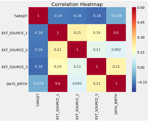
EXT_SOURCE , , EXT_SOURCE . , DAYS_BIRTH EXT_SOURCE_1, , , , .

, . .

plt.figure(figsize = (10, 12))
for i, source in enumerate(['EXT_SOURCE_1', 'EXT_SOURCE_2', 'EXT_SOURCE_3']):
    plt.subplot(3, 1, i + 1)
    sns.kdeplot(app_train.loc[app_train['TARGET'] == 0, source], label = 'target == 0')
    sns.kdeplot(app_train.loc[app_train['TARGET'] == 1, source], label = 'target == 1')
    plt.title('Distribution of %s by Target Value' % source)
    plt.xlabel('%s' % source); plt.ylabel('Density');
plt.tight_layout(h_pad = 2.5)
      
      

        
        
        
      

    
        
        
        
      
      

        
        
        
      

    
    

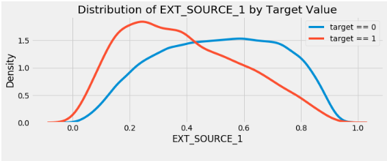
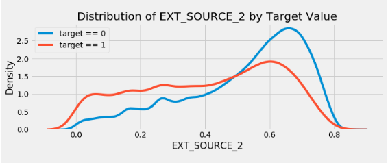
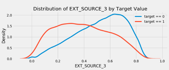
EXT_SOURCE_3 . , . ( ), , , .

EXTSOURCE DAYSBIRTH. – , , . seaborn PairGrid, , 2D .

plot_data = ext_data.drop(columns = ['DAYS_BIRTH']).copy()
plot_data['YEARS_BIRTH'] = age_data['YEARS_BIRTH']
plot_data = plot_data.dropna().loc[:100000, :]

#        
def corr_func(x, y, **kwargs):
    r = np.corrcoef(x, y)[0][1]
    ax = plt.gca()
    ax.annotate("r = {:.2f}".format(r),
                xy=(.2, .8), xycoords=ax.transAxes,
                size = 20)

#    
grid = sns.PairGrid(data = plot_data, size = 3, diag_sharey=False,
                    hue = 'TARGET', 
                    vars = [x for x in list(plot_data.columns) if x != 'TARGET'])
grid.map_upper(plt.scatter, alpha = 0.2)
grid.map_diag(sns.kdeplot)
grid.map_lower(sns.kdeplot, cmap = plt.cm.OrRd_r);
plt.suptitle('Ext Source and Age Features Pairs Plot', size = 32, y = 1.05);
      
      

        
        
        
      

    
        
        
        
      
      

        
        
        
      

    
    

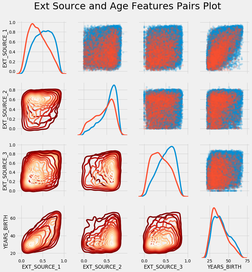
Dans ce graphique, le rouge indique les prêts qui n'ont pas été remboursés et le bleu les prêts qui ont été remboursés. Nous pouvons voir différentes relations dans les données. Il existe en effet une relation linéaire positive modérée entre EXT_SOURCE_1 et YEARS_BIRTH, indiquant que ce trait peut être spécifique à l'âge.

Ceci conclut le premier article. Dans la partie suivante, je parlerai du développement de fonctionnalités supplémentaires basées sur les données disponibles et je montrerai également comment créer un modèle d'apprentissage automatique simple.

Lors de la préparation de l'article, des matériaux provenant de sources ouvertes ont été utilisés:  source_1 ,  source_2 .