Les dates et les heures ne sont pas des objets faciles:
- les mois contiennent un nombre de jours différent;
- les années sont des années bissextiles et non;
- il existe différents fuseaux horaires;
- les heures, les minutes, les jours utilisent différents systèmes de numérotation;
- et bien d'autres nuances.
Ce qui suit est un résumé de certains points rarement mis en évidence dans la documentation, ainsi que des astuces qui vous permettent d'écrire du code rapide et contrôlé.
Un très bref résumé pour les lecteurs de smartphone: sur de grandes quantités de données, nous n'utilisons que des POSIXct
fractions de seconde. Ce sera bien, bien sûr, rapidement.
C'est la continuation d'une série de publications précédentes .
Normes de spécification des dates et des heures
ISO 8601 Éléments de données et formats d'échange - Échange d'informations - Représentation des dates et des heures est une norme internationale couvrant l'échange de données relatives à la date et à l'heure.
Méthodes R de base pour travailler avec le temps
Date
Sys.Date()
print("-----")
x <- as.Date("2019-01-29") # UTC
print(x)
tz(x)
str(x)
dput(x)
print("-----")
dput(as.Date("1970-01-01")) # ! origin
## [1] "2021-04-29" ## [1] "-----" ## [1] "2019-01-29" ## [1] "UTC" ## Date[1:1], format: "2019-01-29" ## structure(17925, class = "Date") ## [1] "-----" ## structure(0, class = "Date")
Le format de date non standard lors de l'initialisation doit être spécifié spécialement
as.Date("04/20/2011", format = "%m/%d/%Y")
## [1] "2011-04-20"
Temps
Il existe deux types de temps de base utilisés dans R: POSIXct
et POSIXlt
.
Les vues externes POSIXct
et POSIXlt
se ressemblent. Et les internes?
z <- Sys.time()
glue(" ",
"POSIXct - {z}",
"POSIXlt - {as.POSIXlt(z)}", "---", .sep = "\n")
glue(" ",
"POSIXct - {capture.output(dput(z))}",
"POSIXlt - {paste0(capture.output(dput(as.POSIXlt(z))), collapse = '')}",
"---", .sep = "\n")
# /
glue(": {year(z)} \n: {minute(z)}\n: {second(z)}\n---")
## ## POSIXct - 2021-04-29 15:18:04 ## POSIXlt - 2021-04-29 15:18:04 ## --- ## ## POSIXct - structure(1619698684.50764, class = c("POSIXct", "POSIXt")) ## POSIXlt - structure(list(sec = 4.50764489173889, min = 18L, hour = 15L, mday = 29L, mon = 3L, year = 121L, wday = 4L, yday = 118L, isdst = 0L, zone = "MSK", gmtoff = 10800L), class = c("POSIXlt", "POSIXt"), tzone = c("", "MSK", "MSD")) ## --- ## : 2021 ## : 18 ## : 4 ## ---
Immédiatement, nous concluons que pour un travail sérieux avec des données (plus de 10 lignes avec le temps), nous l' POSIXlt
oublions comme un mauvais rêve. C'est une structure complexe avec des frais généraux insensés.
POSIXct
unixtimestamp, () ( 0 01.01.1970). .
— online unixtimestamp:
- Epoch Unix Time Stamp Converter
- Epoch & Unix Timestamp Conversion Tools
- currentDate / Time in Millisecondsmillis
z <- 1548802400
as.POSIXct(z, origin = "1970-01-01") # local
as.POSIXct(z, origin = "1970-01-01", tz = "UTC") # in UTC
## [1] "2019-01-30 01:53:20 MSK" ## [1] "2019-01-29 22:53:20 UTC"
. . :
- ISO, (ISO 8601-2019);
- - ;
- .
POSIXct
, - . :
x <- ymd_hms("2014-09-24 15:23:10")
x
x + 0.5
x + 0.5 + 0.6
options(digits.secs=5)
x + 0.45756
options(digits.secs=0)
x
## [1] "2014-09-24 15:23:10 UTC" ## [1] "2014-09-24 15:23:10 UTC" ## [1] "2014-09-24 15:23:11 UTC" ## [1] "2014-09-24 15:23:10.45756 UTC" ## [1] "2014-09-24 15:23:10 UTC"
, .
options(digits.secs=5)
# generate data
df <- data.frame(
timestamp = as_datetime(
round(runif(20, min = now() - seconds(10), max = now()), 0),
tz ="Europe/Moscow")) %>%
mutate(ms = round(runif(n(), 0, 999), 0)) %>%
mutate(value = round(runif(n(), 0, 100), 0))
dput(df)
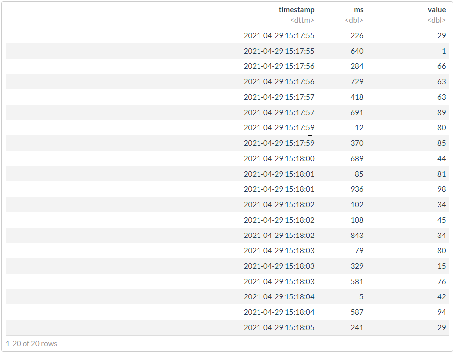
# " "
df %>%
arrange(timestamp, ms)
options(digits.secs=0)
## structure(list(timestamp = structure(c(1619698677, 1619698680, ## 1619698676, 1619698682, 1619698675, 1619698682, 1619698679, 1619698679, ## 1619698684, 1619698683, 1619698684, 1619698677, 1619698682, 1619698683, ## 1619698675, 1619698676, 1619698685, 1619698681, 1619698683, 1619698681 ## ), class = c("POSIXct", "POSIXt"), tzone = "Europe/Moscow"), ## ms = c(418, 689, 729, 108, 226, 843, 12, 370, 5, 581, 587, ## 691, 102, 79, 640, 284, 241, 85, 329, 936), value = c(63, ## 44, 63, 45, 29, 34, 80, 85, 42, 76, 94, 89, 34, 80, 1, 66, ## 29, 81, 15, 98)), class = "data.frame", row.names = c(NA, ## -20L))
# ""
# [magrittr aliases](https://magrittr.tidyverse.org/reference/aliases.html)
df2 <- df %>%
mutate(timestamp = timestamp + ms/1000) %>%
# mutate_at("timestamp", ~`+`(. + ms/1000)) %>%
select(-ms) %>%
df2 %>% arrange(timestamp)

#
dt <- as.data.table(df2)
bench::mark(
naive = dplyr::arrange(df, timestamp, ms),
smart = dplyr::arrange(df2, timestamp),
dt = dt[order(timestamp)],
check = FALSE,
relative = TRUE,
min_iterations = 1000
)
## # A tibble: 3 x 6 ## expression min median `itr/sec` mem_alloc `gc/sec` ## <bch:expr> <dbl> <dbl> <dbl> <dbl> <dbl> ## 1 naive 11.9 11.8 1 1.06 1 ## 2 smart 11.1 11.0 1.06 1 1.06 ## 3 dt 1 1 11.6 494. 1.22
.
data <- c("05102019210003657", "05102019210003757", "05102019210003857")
dmy_hms(stri_c(stri_sub(data, to = 14L), ".", stri_sub(data, from = 15L)), tz = "Europe/Moscow")
#
data2 <- data %>%
sample(10^6, replace = TRUE)
bench::mark(
stri_sub = stri_c(stri_sub(data2, to = 14L), ".", stri_sub(data2, from = 15L)),
stri_replace = stri_replace_first_regex(data2, pattern = "(^.{14})(.*)", replacement = "$1.$2"),
re2_replace = re2_replace(data2, pattern = "(^.{14})(.*)", replacement = "\\1.\\2", parallel = TRUE)
)
## [1] "2019-10-05 21:00:03 MSK" "2019-10-05 21:00:03 MSK" ## [3] "2019-10-05 21:00:03 MSK" ## # A tibble: 3 x 6 ## expression min median `itr/sec` mem_alloc `gc/sec` ## <bch:expr> <bch:tm> <bch:tm> <dbl> <bch:byt> <dbl> ## 1 stri_sub 214ms 222ms 4.10 22.89MB 5.47 ## 2 stri_replace 653ms 653ms 1.53 7.63MB 0 ## 3 re2_replace 409ms 413ms 2.42 15.29MB 1.21
lubridate
x <- ymd(20101215)
print(x)
class(x)
## [1] "2010-12-15" ## [1] "Date"
lubridate
ymd(20101215) == mdy("12/15/10")
## [1] TRUE
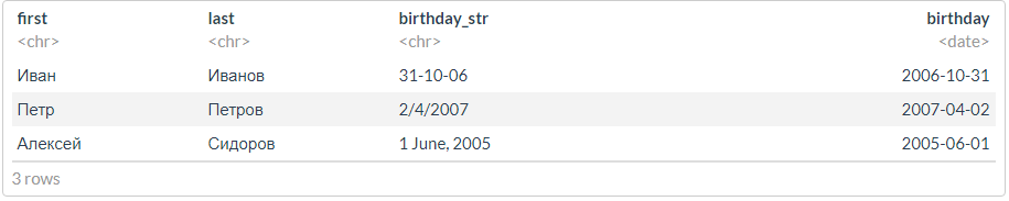
df <- tibble(first = c("", "", ""),
last = c("", "", ""),
birthday_str = c("31-10-06", "2/4/2007", "1 June, 2005")) %>%
mutate(birthday = dmy(birthday_str))
df
, ?
# lubridate
options(lubridate.verbose = TRUE)
# : ..
df <- tibble(time_str = c("08.05.19 12:04:56", "09.05.19 12:05", "12.05.19 23"))
lubridate::dmy_hms(df$time_str, tz = "Europe/Moscow")
print("---------------------")
lubridate::dmy(df$time_str, tz = "Europe/Moscow")
## [1] "2019-05-08 12:04:56 MSK" NA ## [3] NA ## [1] "---------------------" ## [1] NA NA NA
# lubridate
options(lubridate.verbose = TRUE)
lubridate::dmy_hms(df$time_str, truncated = 3, tz = "Europe/Moscow")
## [1] "2019-05-08 12:04:56 MSK" "2019-05-09 12:05:00 MSK" ## [3] "2019-05-12 23:00:00 MSK"
# lubridate
options(lubridate.verbose = TRUE)
# : ..
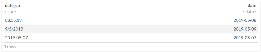
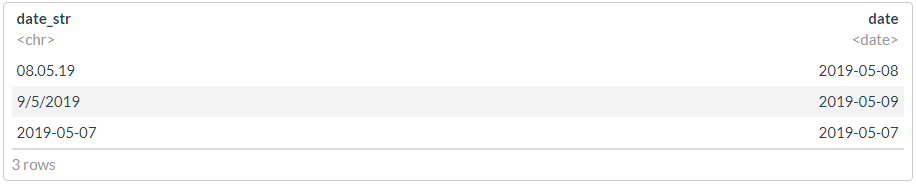
df <- tibble(date_str = c("08.05.19", "9/5/2019", "2019-05-07"))
#
glimpse(dmy(df$date_str))
print("---------------------")
#
glimpse(ymd(df$date_str))
print("---------------------")
## Date[1:3], format: "2019-05-08" "2019-05-09" NA ## [1] "---------------------" ## Date[1:3], format: "2008-05-19" NA "2019-05-07" ## [1] "---------------------"
? , , , - .
df %>% mutate(date = dplyr::coalesce(dmy(date_str), ymd(date_str)))
df1 <- df
df1$date <- dmy(df1$date_str)
idx <- is.na(df1$date)
print("---------------------")
idx
df1$date[idx] <- ymd(df1$date_str[idx])
print("---------------------")
df1
## [1] "---------------------" ## [1] FALSE FALSE TRUE ## [1] "---------------------"
"" :
POSIXct
options(lubridate.verbose = FALSE)
date1 <- ymd_hms("2011-09-23-03-45-23")
date2 <- ymd_hms("2011-10-03-21-02-19")
# ?
as.numeric(date2) - as.numeric(date1) # ,
(date2 - date1) %>% dput()
difftime(date2, date1)
difftime(date2, date1, unit="mins")
difftime(date2, date1, unit="secs")
## [1] 926216 ## structure(10.7200925925926, class = "difftime", units = "days") ## Time difference of 10.72009 days ## Time difference of 15436.93 mins ## Time difference of 926216 secs
date1 <- ymd_hms("2019-01-30 00:00:00")
date1
date1 - days(1)
date1 + days(1)
date1 + days(2)
## [1] "2019-01-30 UTC" ## [1] "2019-01-29 UTC" ## [1] "2019-01-31 UTC" ## [1] "2019-02-01 UTC"
—
date1 - months(1)
date1 + months(1) # !!!
## [1] "2018-12-30 UTC" ## [1] NA
. , .
date1 %m-% months(1)
date1 %m+% months(1)
date1 %m+% months(1) %m-% months(1)
## [1] "2018-12-30 UTC" ## [1] "2019-02-28 UTC" ## [1] "2019-01-28 UTC"
date1 <- ymd_hms("2019-01-30 01:00:00")
date1 %T>% print() %>% dput()
with_tz(date1, tzone = "Europe/Moscow") %T>% print() %>% dput()
force_tz(date1, tzone = "Europe/Moscow") %T>% print() %>% dput()
## [1] "2019-01-30 01:00:00 UTC" ## structure(1548810000, class = c("POSIXct", "POSIXt"), tzone = "UTC") ## [1] "2019-01-30 04:00:00 MSK" ## structure(1548810000, class = c("POSIXct", "POSIXt"), tzone = "Europe/Moscow") ## [1] "2019-01-30 01:00:00 MSK" ## structure(1548799200, class = c("POSIXct", "POSIXt"), tzone = "Europe/Moscow")
, , ? , hms
. .
hms_str <- "03:22:14"
as_hms(hms_str)
dput(as_hms(hms_str))
print("-------")
x <- as_hms(hms_str) * 15
x
str(x)
# seconds_to_period(period_to_seconds(x))
seconds_to_period(x) %T>% dput() %>% print()
## 03:22:14 ## structure(12134, units = "secs", class = c("hms", "difftime")) ## [1] "-------" ## Time difference of 182010 secs ## 'difftime' num 182010 ## - attr(*, "units")= chr "secs" ## new("Period", .Data = 30, year = 0, month = 0, day = 2, hour = 2, ## minute = 33) ## [1] "2d 2H 33M 30S"
— . .
( Clickhouse) , , unixtimestamp UTC. , .
:
- . timestamp, , , , , .
- ( ). , , , .
- unixtimestamp UTC , . (!).
- , timestamp. ,
X-1
X+1
, .
, 0.
.
(, ) . , :
- , ;
- ;
- ;
- ( );
- ;
-
double
; - ;
- .
-- ClickHouse
SELECT DISTINCT
store, pos,
timestamp, ms,
concat(toString(store), '-', toString(pos)) AS pos_uid,
toFloat64(timestamp) + (ms / 1000) AS timestamp
flog.info(paste("SQL query:", sql_req))
tic(" CH")
raw_df <- dbGetQuery(conn, stri_encode(sql_req, to = "UTF-8")) %>%
mutate_if(is.character, `Encoding<-`, "UTF-8") %>%
as_tibble() %>%
mutate_at(vars(timestamp), anytime::anytime, tz = "Europe/Moscow") %>%
mutate_at("event", as.factor)
flog.info(capture.output(toc()))
DBI::dbDisconnect(conn)
data.frame
#
df -> as_tibble(_df) %>%
map(pryr::object_size) %>%
unlist() %>%
enframe() %>%
arrange(desc(value)) %>%
mutate_at("value", fs::as_fs_bytes) %>%
mutate(ratio = formattable::percent(value / sum(value), 2)) %>%
add_row(name = "TOTAL", value = sum(.$value))
,
- Epoch & Unix Timestamp Conversion Tools
- currentdate/time in millisecondsmillis
- Functions for working with dates and times
, , , . .
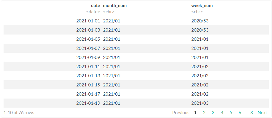
df <- seq.Date(from = as.Date("2021-01-01"),
to = as.Date("2021-05-31"),
by = "2 days") %>%
# sample(20, replace = FALSE) %>%
tibble(date = .)
# //
# 1
df %>%
mutate(month_num = stri_c(lubridate::year(date),
sprintf("%02d", lubridate::month(date)),
sep = "/"),
week_num = stri_c(lubridate::isoyear(date),
sprintf("%02d", lubridate::isoweek(date)),
sep = "/")
)
# //
# 2,
# , !!!
df %>%
mutate(month_num = format(date, "%Y/%m (%a) ISO week %V"))
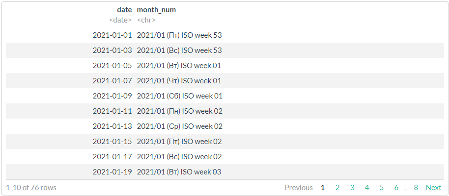
# //
# 3,
# strptime (ISO 8601) ICU
# https://man7.org/linux/man-pages/man3/strptime.3.html
stri_datetime_fstr("%Y/%m (%a) week %V")
# ggthemes::tableau_color_pal("Tableau 20")(20) %>% scales::show_col()
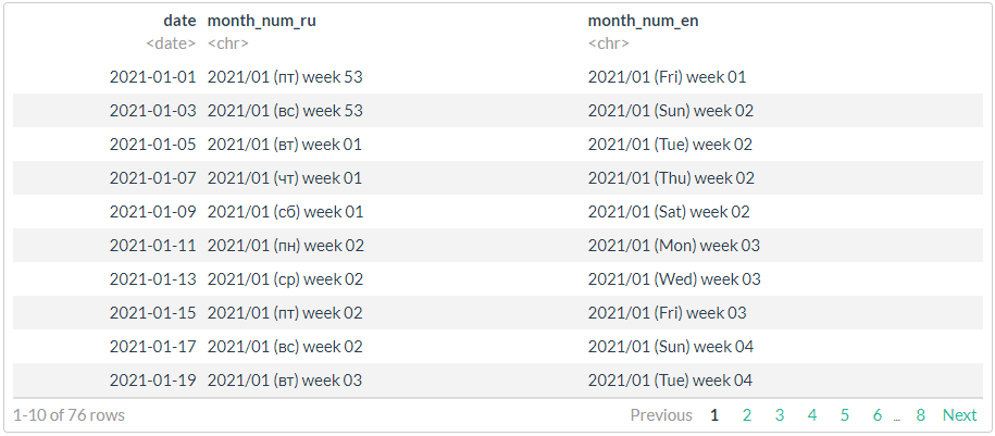
# , !!!
df %>%
mutate(
month_num_ru = stri_datetime_format(
date, "yyyy'/'MM' ('ccc') week 'ww", locale = "ru", tz = "UTC"),
month_num_en = stri_datetime_format(
date, "yyyy'/'MM' ('ccc') week 'ww", locale = "en", tz = "UTC"))
. .
stri_datetime_format(today(), "LLLL", locale="ru@calendar=Persian")
stri_datetime_format(today(), "LLLL", locale="ru@calendar=Indian")
stri_datetime_format(today(), "LLLL", locale="ru@calendar=Hebrew")
stri_datetime_format(today(), "LLLL", locale="ru@calendar=Islamic")
stri_datetime_format(today(), "LLLL", locale="ru@calendar=Coptic")
stri_datetime_format(today(), "LLLL", locale="ru@calendar=Ethiopic")
stri_datetime_format(today(), "dd MMMM yyyy", locale="ru")
stri_datetime_format(today(), "LLLL d, yyyy", locale="ru")
## [1] "" ## [1] "" ## [1] "" ## [1] "" ## [1] "" ## [1] "" ## [1] "29 2021" ## [1] " 29, 2021"
.
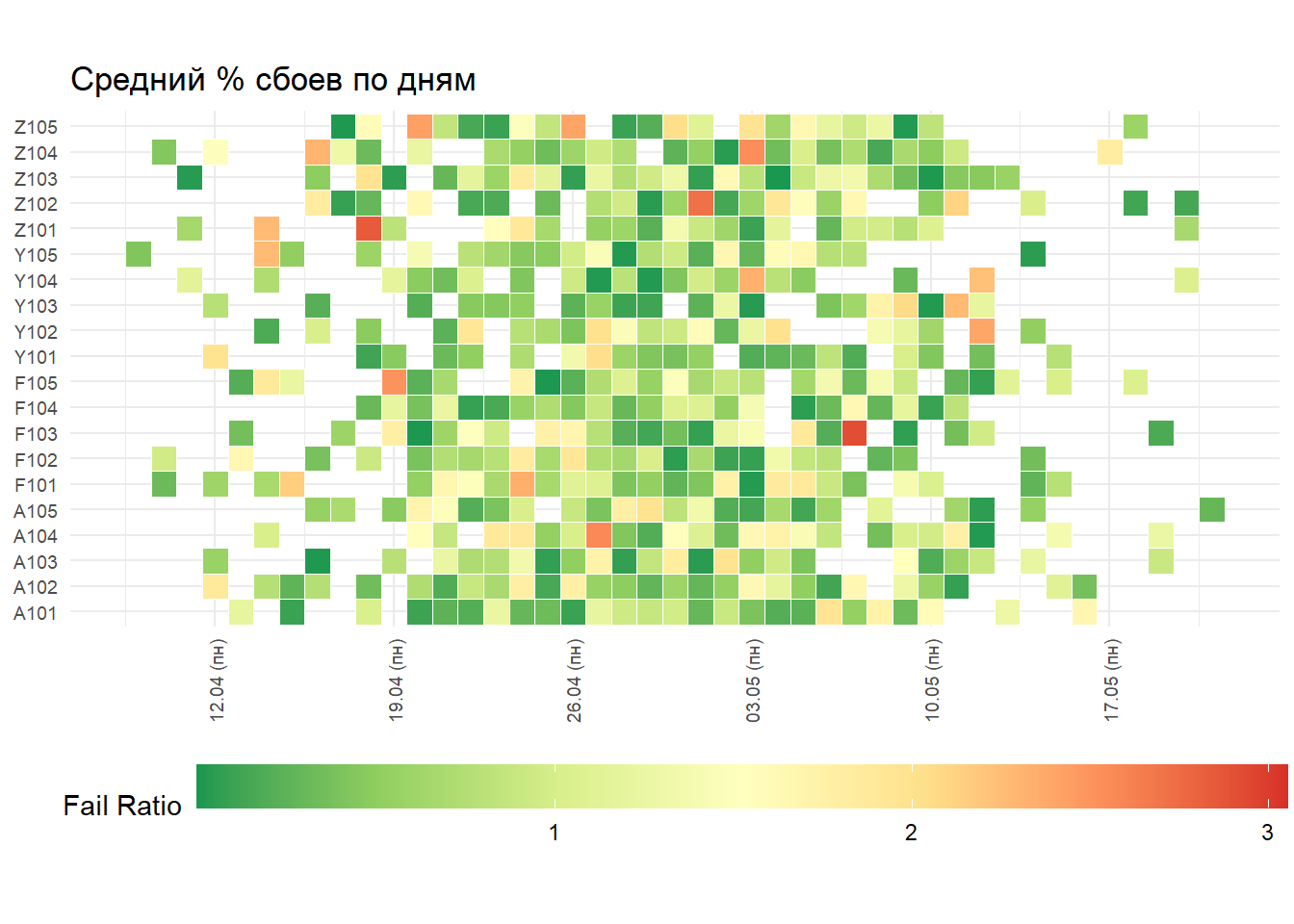
#
map_tbl <- tibble(
date = as_date(Sys.time() + rnorm(10^3, mean = 0, sd = 60 * 60 * 24 * 7))) %>%
mutate(store = stri_c(sample(c("A", "F", "Y", "Z"), n(), replace = TRUE),
sample(101:105, n(), replace = TRUE))) %>%
mutate(store_fct = as.factor(store)) %>%
mutate(fail_ratio = abs(rnorm(n(), mean = 0.3, sd = 1)))
my_date_format <- function (format = "dd MMMM yyyy", tz = "Europe/Moscow")
{
scales:::force_all(format, tz)
# stri_datetime_fstr("%d.%m%n%A")
# stri_datetime_fstr("%d.%m (%a)")
function(x) stri_datetime_format(x, format, locale = "ru", tz = tz)
}
# ,
gp <- map_tbl %>%
ggplot(aes(x = date, y = store_fct, fill = fail_ratio)) +
geom_tile(color = "white", size = 0.1) +
# scale_fill_distiller(palette = "RdYlGn", name = "Fail Ratio", label = comma) +
# scale_fill_distiller(palette = "RdYlGn", name = "Fail Ratio", guide = guide_legend(keywidth = unit(4, "cm"))) +
scale_fill_distiller(palette = "RdYlGn", name = "Fail Ratio") +
scale_x_date(breaks = scales::date_breaks("1 week"), labels = my_date_format("dd'.'MM' ('ccc')'")) +
coord_equal() +
labs(x = NULL, y = NULL, title = " % ") +
theme_minimal() +
theme(plot.title = element_text(hjust = 0)) +
theme(axis.ticks = element_blank()) +
theme(axis.text = element_text(size = 7)) +
theme(axis.text.x = element_text(angle = 90, vjust = 0.5)) +
theme(legend.position = "bottom") +
theme(legend.key.width = unit(3, "cm"))
gp
base_df <- tibble(
start = Sys.time() + rnorm(10^3, mean = 0, sd = 60 * 24 * 3)) %>%
mutate(finish = start + rnorm(n(), mean = 100, sd = 60)) %>%
mutate(user_id = sample(as.character(1000:1100), n(), replace = TRUE)) %>%
arrange(user_id, start)
dt <- as.data.table(base_df, key = c("user_id", "start")) %>%
.[, c("start", "finish") := lapply(.SD, as.numeric),
.SDcols = c("start", "finish")]
df <- group_by(base_df, user_id)
bench::mark(
dplyr_v1 = df %>% transmute(delta_t = as.numeric(difftime(finish, start, units = "secs"))) %>% ungroup(),
dplyr_v2 = ungroup(df) %>% transmute(delta_t = as.numeric(difftime(finish, start, units = "secs"))),
dplyr_v3 = dt %>% transmute(delta_t = finish - start),
dt_v1 = dt[, .(delta_t = finish - start), by = user_id],
dt_v2 = dt[, .(delta_t = finish - start)],
check = FALSE # all_equal
)
## # A tibble: 5 x 6 ## expression min median `itr/sec` mem_alloc `gc/sec` ## <bch:expr> <bch:tm> <bch:tm> <dbl> <bch:byt> <dbl> ## 1 dplyr_v1 4.3ms 4.86ms 200. 103.1KB 11.4 ## 2 dplyr_v2 2.17ms 2.46ms 380. 17.9KB 6.24 ## 3 dplyr_v3 1.67ms 1.77ms 527. 29.8KB 8.51 ## 4 dt_v1 410.4us 438.7us 2139. 90.8KB 8.35 ## 5 dt_v2 304.4us 335.3us 2785. 264.6KB 8.38
: //. , , ?
Exemple de code. N'oubliez pas qu'un certain nombre de fonctions fonctionnent en tenant compte des paramètres régionaux de la machine sur laquelle le code est exécuté. Et si votre mois est imprimé en russe, cela ne garantit pas (si vous n'utilisez pas de méthodes) un comportement similaire sur une autre machine ou un autre système d'exploitation.
# https://stackoverflow.com/questions/16347731/how-to-change-the-locale-of-r
# https://jangorecki.gitlab.io/data.cube/library/stringi/html/stringi-locale.html
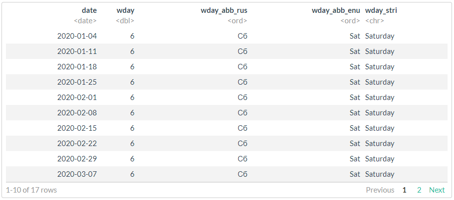
df <- as.Date("2020-01-01") %>%
seq.Date(to = . + months(4), by = "1 day") %>%
tibble(date = .) %>%
mutate(wday = lubridate::wday(date, week_start = 1),
wday_abb_rus = lubridate::wday(date, label = TRUE, week_start = 1),
wday_abb_enu = lubridate::wday(date, label = TRUE, week_start = 1, locale = "English"),
wday_stri = stringi::stri_datetime_format(date, "EEEE", locale = "en"))
#
filter(df, wday == 6)
PS La plupart des tests sont à titre d'exemple uniquement. Vous pouvez l'exécuter sur vos machines, les chiffres seront complètement différents, mais la nature de la dépendance et le rapport doivent être à peu près les mêmes.
Article précédent - "R vs Python dans une boucle productive" .