Je ne sais pas pour vous, mais les statistiques n’ont pas été faciles pour moi. De plus, il a été «donné» - c'est toujours dit à haute voix. Oui, il s'est avéré que vous pouvez aller assez longtemps sur les manuels de formation, en explorant d'une manière ou d'une autre la signification des formules à quatre étages, et parfois même en ne comprenant pas les résultats, mais quand même y aller. Aller et ne pas avoir de plaisir - tout semble clair, mais le sentiment que vous n'êtes "pas tout à fait dans le sujet" ne part toujours pas. Pendant un moment, j'ai essayé de lire des livres sur R et non pas que ce serait complètement infructueux, mais pas non plus "feu". J'ai trouvé le livre le plus cool "Statistics for All" de Sarah Boslaf, lisez-le ... il y avait encore quelques nuances dont le sens n'est pas entièrement compris.
En général, comme vous l'avez deviné, cet article est issu de la série "J'essaie d'expliquer sur mes doigts pour le comprendre moi-même". Donc, si vous n'êtes pas indifférent aux statistiques, alors s'il vous plaît, sous cat.
, , . , :
" " . . , . . ;
" " . . . , , " ". , - , " " . , , - - . :
" " . . . . "", . .
" " . , , , . , , , . , . , , . , , . .
, ", , , ", , , "".
(- , ) " - ". NumPy, matplotlib, seaborn SciPy - . , .
... , - :
import numpy as np
from scipy import stats
import matplotlib.pyplot as plt
#import seaborn as sns
from pylab import rcParams
#sns.set()
rcParams['figure.figsize'] = 10, 6
%config InlineBackend.figure_format = 'svg'
np.random.seed(42)
, , , , , . :
norm_rv = stats.norm(loc=30, scale=5)
samples = np.trunc(norm_rv.rvs(365))
samples[:30]
array([32., 29., 33., 37., 28., 28., 37., 33., 27., 32., 27., 27., 31.,
20., 21., 27., 24., 31., 25., 22., 37., 28., 30., 22., 27., 30.,
24., 31., 26., 28.])
:
samples.mean(), samples.std()
(29.52054794520548, 4.77410133275075)
, -  .
.
, , :
sns.histplot(x=samples, discrete=True);

, , 
 . , , ? ? , , :
norm_rv = stats.norm(loc=30, scale=5)
beta_rv = stats.beta(a=5, b=5, loc=14, scale=32)
gamma_rv = stats.gamma(a = 20, loc = 7, scale=1.2)
tri_rv = stats.triang(c=0.5, loc=17, scale=26)
x = np.linspace(10, 50, 300)
sns.lineplot(x = x, y = norm_rv.pdf(x), color='r', label='norm')
sns.lineplot(x = x, y = beta_rv.pdf(x), color='g', label='beta')
sns.lineplot(x = x, y = gamma_rv.pdf(x), color='k', label='gamma')
sns.lineplot(x = x, y = tri_rv.pdf(x), color='b', label='triang')
sns.histplot(x=samples, discrete=True, stat='probability',
alpha=0.2);

?
, :
;
- ;
;
;
;
, .
, , ( , - . ?). , , , .. . ,  , . , :
unif_rv = stats.uniform(loc=0, scale=4)
unif_rv.rvs()
0.8943833540778106
, - -- :
unif_rv.rvs(size=3)
array([3.85289016, 0.0486179 , 3.87951531])
, 15 , . , :
- , - .. ;
, , , - .. ;
, , , , - - .. .
15 :  , , ,
, , ,  :
:

 , -
, -  ? 10 :
Y_samples = [unif_rv.rvs(size=15).sum() for i in range(10000)]
sns.histplot(x=Y_samples);

, ? , , : .
, , :
. , ;
- . - ;
. ;
. , ;
. ?;
, . , .
,  , . , , :

:

 ? , . , 365- , , , .
Z-
, . , . ,  , , 40 , 35 .
? , ? , , ,  , 27, 31, 35 , 23 38 . , 365 , 20 45 .
  , , - 25 35 . , :
N = 5000
t_data = norm_rv.rvs(N)
t_data[(25 < t_data) & (t_data < 35)].size/N
0.7008
- 25 35 . 40 ?
t_data[t_data > 40].size/N
0.0248
40 . 40 . , :
0.02**3
8.000000000000001e-06
, - . Z-.
Z- :

 - , .. -
  , ,
, , 
 . , .. , 30 5 . Z- :

? , . Z-? "":
fig, ax = plt.subplots()
x = np.linspace(norm_rv.ppf(0.001), norm_rv.ppf(0.999), 200)
ax.vlines(40.5, 0, 0.1, color='k', lw=2)
sns.lineplot(x=x, y=norm_rv.pdf(x), color='r', lw=3)
sns.histplot(x=samples, stat='probability', discrete=True);

samples, , . . 40 . , . - , .. , , 5000 , , :
np.random.seed(42)
N = 10000
values = np.trunc(norm_rv.rvs(N))
fig, ax = plt.subplots()
v_le_41 = np.histogram(values, np.arange(9.5, 41.5))
v_ge_40 = np.histogram(values, np.arange(40.5, 51.5))
ax.bar(np.arange(10, 41), v_le_41[0]/N, color='0.8')
ax.bar(np.arange(41, 51), v_ge_40[0]/N)
p = np.sum(v_ge_40[0]/N)
ax.set_title('P(Y>40min) = {:.3}'.format(p))
ax.vlines(40.5, 0, 0.08, color='k', lw=1);
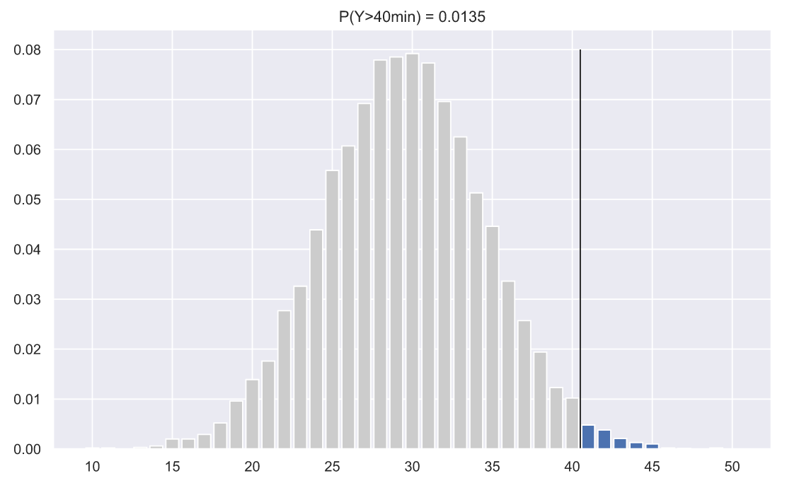
- . , , . , , , . , , 40 :
fig, ax = plt.subplots()
x = np.linspace(norm_rv.ppf(0.0001), norm_rv.ppf(0.9999), 300)
ax.plot(x, norm_rv.pdf(x))
ax.fill_between(x[x>41], norm_rv.pdf(x[x>41]), np.zeros(len(x[x>41])))
p = 1 - norm_rv.cdf(41)
ax.set_title('P(Y>40min) = {:.3}'.format(p))
ax.hlines(0, 10, 50, lw=1, color='k')
ax.vlines(41, 0, 0.08, color='k', lw=1);

. , , - , "", - , . , - , . 40 , .. 41, 42, 43 .. . 41.0. , SciPy , , - . , , - , : , , .. , Z-.
, - 
 . 99 143 , ? , , :
fig, ax = plt.subplots(nrows=1, ncols=2, figsize = (12, 5))
nrv_hobbit = stats.norm(91, 8)
nrv_gnome = stats.norm(134, 6)
for i, (func, h) in enumerate(zip((nrv_hobbit, nrv_gnome), (99, 143))):
x = np.linspace(func.ppf(0.0001), func.ppf(0.9999), 300)
ax[i].plot(x, func.pdf(x))
ax[i].fill_between(x[x>h], func.pdf(x[x>h]), np.zeros(len(x[x>h])))
p = 1 - func.cdf(h)
ax[i].set_title('P(H > {} ) = {:.3}'.format(h, p))
ax[i].hlines(0, func.ppf(0.0001), func.ppf(0.9999), lw=1, color='k')
ax[i].vlines(h, 0, func.pdf(h), color='k', lw=2)
ax[i].set_ylim(0, 0.07)
fig.suptitle(' , ', fontsize = 20);

, , , ( ), . , . "".
Z-:

fig, ax = plt.subplots()
N_rv = stats.norm()
x = np.linspace(N_rv.ppf(0.0001), N_rv.ppf(0.9999), 300)
ax.plot(x, N_rv.pdf(x))
ax.hlines(0, -4, 4, lw=1, color='k')
ax.vlines(1, 0, 0.4, color='r', lw=2, label='')
ax.vlines(1.5, 0, 0.4, color='g', lw=2, label='')
ax.legend();

Z- , "", ..  , Z- . , , , Z- . :

, .
Z- "" , Z- . :

, : , , ; , Z- . Z-, , Z- .
, - - . , . , , Z- - () , . . , , , . - .
Z-
, . Z- 40 :

, , :
fig, ax = plt.subplots()
N_rv = stats.norm()
x = np.linspace(N_rv.ppf(0.0001), N_rv.ppf(0.9999), 300)
ax.plot(x, N_rv.pdf(x))
ax.hlines(0, -4, 4, lw=1, color='k')
ax.vlines(2, 0, 0.4, color='g', lw=2);

 , . , , . , - !
, - . 365- , , .. ,  . . , , , . 5000 :
sns.histplot(np.trunc(norm_rv.rvs(size=(N, 3))).mean(axis=1),
bins=np.arange(19, 42));

, 40 - . :
;
- , .. - , .
Z- (Z = 2), ( ) :
1 - N_rv.cdf(2)
0.02275013194817921
, 40 :
(1 - N_rv.cdf(2))**3
1.1774751750476762e-05
Z-, - Z-:

 - ,
- , 
 ,
,  - .
- .
35 , Z- :

Z-, Z- , . , ,

[25; 35] . :
N = 10000
means = np.trunc(norm_rv.rvs(size=(N, 3))).mean(axis=1)
means[(means>=25)&(means<=35)].size/N
0.9241
N = 10000
fig, ax = plt.subplots()
means = np.trunc(norm_rv.rvs(size=(N, 3))).mean(axis=1)
h = np.histogram(means, np.arange(19, 41))
ax.bar(np.arange(20, 25), h[0][0:5]/N, color='0.5')
ax.bar(np.arange(25, 36), h[0][5:16]/N)
ax.bar(np.arange(36, 41), h[0][16:22]/N, color='0.5')
p = np.sum(h[0][6:16]/N)
ax.set_title('P(25min < Y < 35min) = {:.3}'.format(p))
ax.vlines([24.5 ,35.5], 0, 0.08, color='k', lw=1);

, :
x, n, mu, sigma = 35, 3, 30, 5
z = abs((x - mu)/(sigma/n**0.5))
N_rv = stats.norm()
fig, ax = plt.subplots()
x = np.linspace(N_rv.ppf(0.0001), N_rv.ppf(0.9999), 300)
ax.plot(x, N_rv.pdf(x))
ax.hlines(0, x.min(), x.max(), lw=1, color='k')
ax.vlines([-z, z], 0, 0.4, color='g', lw=2)
x_z = x[(x>-z) & (x<z)] # & (x<z)
ax.fill_between(x_z, N_rv.pdf(x_z), np.zeros(len(x_z)), alpha=0.3)
p = N_rv.cdf(z) - N_rv.cdf(-z)
ax.set_title('P({:.3} < z < {:.3}) = {:.3}'.format(-z, z, p));

, Z- -  , -
, -  . 5, 30 100 , , [29; 31]? :
fig, ax = plt.subplots(nrows=1, ncols=3, figsize = (12, 4))
for i, n in enumerate([5, 30, 100]):
x, mu, sigma = 31, 30, 5
z = abs((x - mu)/(sigma/n**0.5))
N_rv = stats.norm()
x = np.linspace(N_rv.ppf(0.0001), N_rv.ppf(0.9999), 300)
ax[i].plot(x, N_rv.pdf(x))
ax[i].hlines(0, x.min(), x.max(), lw=1, color='k')
ax[i].vlines([-z, z], 0, 0.4, color='g', lw=2)
x_z = x[(x>-z) & (x<z)] # & (x<z)
ax[i].fill_between(x_z, N_rv.pdf(x_z), np.zeros(len(x_z)), alpha=0.3)
p = N_rv.cdf(z) - N_rv.cdf(-z)
ax[i].set_title('n = {}, z = {:.3}, p = {:.3}'.format(n, z, p));
fig.suptitle(r'Z- $\bar{x} = 31$', fontsize = 20, y=1.02);

5 [29;31] , . 30 . - 1 .
, : 30 , 31 5, 30 100 ? , n=5 , , ,  .
.  ,
, 
 . ? , 100 31 , , 30 .
, 3 ? ? - . 40 , Z- 3.81, 1:
x, n, mu, sigma = 41, 3, 30, 5
z = abs((x - mu)/(sigma/3**0.5))
N_rv = stats.norm()
fig, ax = plt.subplots()
x = np.linspace(N_rv.ppf(1e-5), N_rv.ppf(1-1e-5), 300)
ax.plot(x, N_rv.pdf(x))
ax.hlines(0, x.min(), x.max(), lw=1, color='k')
ax.vlines([-z, z], 0, 0.4, color='g', lw=2)
x_z = x[(x>-z) & (x<z)] # & (x<z)
ax.fill_between(x_z, N_rv.pdf(x_z), np.zeros(len(x_z)), alpha=0.3)
p = N_rv.cdf(z) - N_rv.cdf(-z)
ax.set_title('P({:.3} < z < {:.3}) = {:.3}'.format(-z, z, p));

, , , 
 10 . :
"" ;
.
? .
p-value
Z- , 
 , . ,
, . ,  . Z-, . ,
 [29;31] 0.35. 1−0.35=0.65. ,
 , - .
, - .
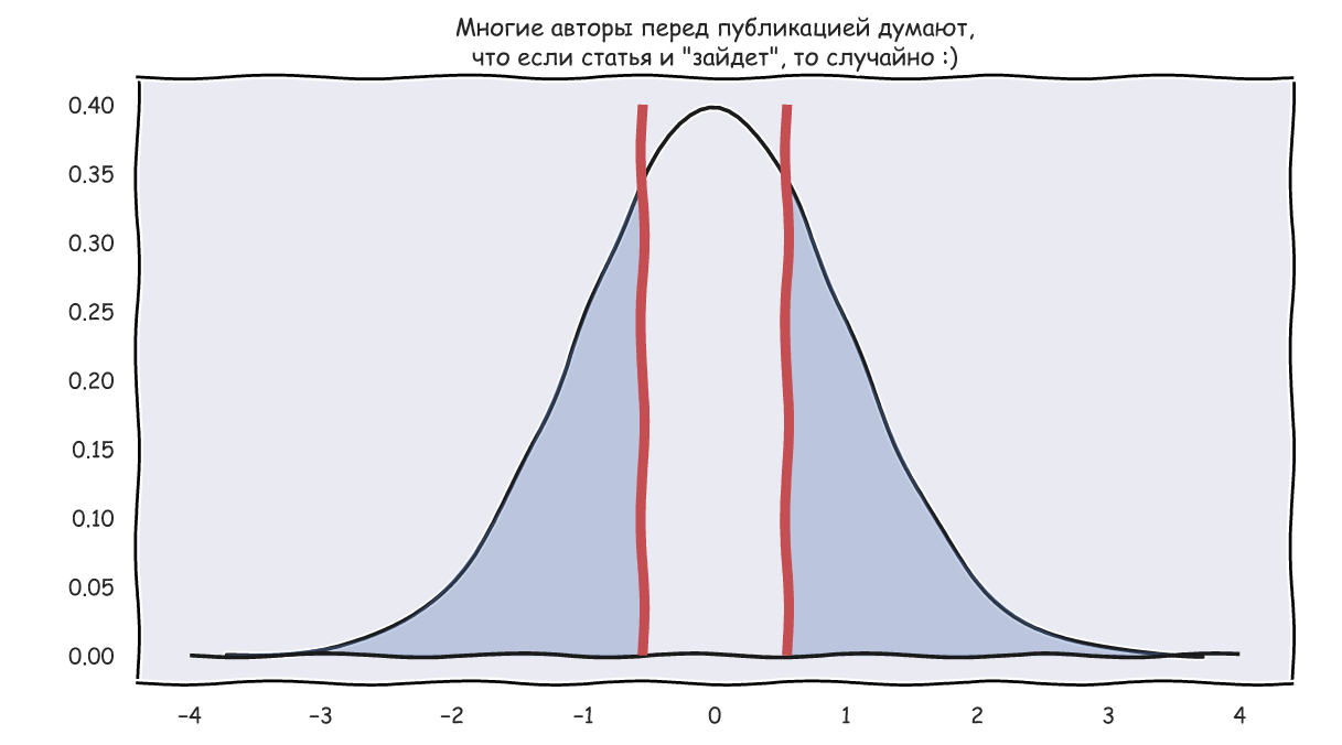
, 0.65, - p-value , Z-, :
x, n, mu, sigma = 31, 5, 30, 5
z = abs((x - mu)/(sigma/n**0.5))
N_rv = stats.norm()
fig, ax = plt.subplots()
x = np.linspace(N_rv.ppf(0.0001), N_rv.ppf(0.9999), 300)
ax.plot(x, N_rv.pdf(x))
ax.hlines(0, x.min(), x.max(), lw=1, color='k')
ax.vlines([-z, z], 0, 0.4, color='g', lw=2)
x_le_z, x_ge_z = x[x<-z], x[x>z]
ax.fill_between(x_le_z, N_rv.pdf(x_le_z), np.zeros(len(x_le_z)), alpha=0.3, color='b')
ax.fill_between(x_ge_z, N_rv.pdf(x_ge_z), np.zeros(len(x_ge_z)), alpha=0.3, color='b')
p = N_rv.cdf(z) - N_rv.cdf(-z)
ax.set_title('P({:.3} < z < {:.3}) = {:.3}'.format(-z, z, p));

p-value , . p-value , .. . - , p-value , . , , ,  0.05, , p-value . , ,
  . ,
. ,  , , 5 , ..
  :
:
1 - (N_rv.cdf(5) - N_rv.cdf(-5))
5.733031438470704e-07
, , . , , , . , , - "" . , ( ) . , . , , , .
, , . , ,  , 31 , 30 , 100 .
, , Z- : , , , .
Cela ne semble pas très plausible, mais jetons un coup d'œil. Nous générerons 1000 valeurs à partir des distributions uniformes, exponentielles et de Laplace, puis, séquentiellement, pour chaque distribution, nous construirons des kde-graphes des distributions de la valeur moyenne d'échantillons de différentes tailles:
Code GIF
import matplotlib.animation as animation
fig, axes = plt.subplots(nrows=2, ncols=3, figsize = (12, 7))
unif_rv = stats.uniform(loc=10, scale=10)
exp_rv = stats.expon(loc=10, scale=1.5)
lapl_rv = stats.laplace(loc=15)
np.random.seed(42)
unif_data = unif_rv.rvs(size=1000)
exp_data = exp_rv.rvs(size = 1000)
lapl_data = lapl_rv.rvs(size=1000)
title = ['Uniform', 'Exponential', 'Laplace']
data = [unif_data, exp_data, lapl_data]
y_max = [60, 310, 310]
n = [3, 10, 30, 50]
for i, ax in enumerate(axes[0]):
sns.histplot(data[i], bins=20, alpha=0.4, ax=ax)
ax.vlines(data[i].mean(), 0, y_max[i], color='r')
ax.set_xlim(10, 20)
ax.set_title(title[i])
def animate(i):
for ax in axes[1]:
ax.clear()
for j in range(3):
rand_idx = np.random.randint(0, 1000, size=(1000, n[i]))
means = data[j][rand_idx].mean(axis=1)
sns.kdeplot(means, ax=axes[1][j])
axes[1][j].vlines(means.mean(), 0, 2, color='r')
axes[1][j].set_xlim(10, 20)
axes[1][j].set_ylim(0, 2.1)
axes[1][j].set_title('n = ' + str(n[i]))
fig.set_figwidth(15)
fig.set_figheight(8)
return axes[1][0], axes[1][1],axes[1][2]
dist_animation = animation.FuncAnimation(fig,
animate,
frames=np.arange(4),
interval = 200,
repeat = False)
# gif :
dist_animation.save('dist_means.gif',
writer='imagemagick',
fps=1)
Bien sûr, l'image n'est pas du tout une preuve, mais si vous le souhaitez, vous pouvez exécuter vous-même les tests de normalité. Cependant, dans le prochain article, nous allons simplement faire des tests et prouver des hypothèses.
En général, merci pour votre attention. J'appuie sur F5 et j'attends avec impatience vos et vos commentaires.