➖ 🎙️ 🗒️ Matrice-Rematrix 👃🏻 👨🏿‍✈️ 🎅🏻

Le travail d'un réseau de neurones est basé sur la manipulation matricielle. Pour la formation, une variété de méthodes sont utilisées, dont beaucoup sont issues de la méthode de descente de gradient, où il est nécessaire de pouvoir manipuler des matrices, pour calculer des gradients (dérivés par rapport aux matrices). Si vous regardez sous le capot d'un réseau de neurones, vous pouvez voir des chaînes de matrices, qui semblent souvent intimidantes. En termes simples, «la matrice nous attend tous». Il est temps de mieux se connaître.

Pour ce faire, nous allons suivre les étapes suivantes:

Considérons les manipulations avec des matrices: transposition, multiplication, gradient;
;
.

NumPy . , , , , . , , , - , , , . , - : , .

-

- , , , . , , , Google TensorFlow.

, , , , , $a_ {i}$ , i = 0, 1, 2, ..., n-1 ; - .

import numpy as np #   numpy
a=np.array([1,2,5])
a.ndim #  ,   = 1
a.shape #      (3,)
a.shape[0] #      = 3

$a_ {i} \ cdot b_ {i} = a_ {0} \ cdot b_ {0} + a_ {1} \ cdot b_ {1} + a_ {2} \ cdot b_ {2}$ . , , 0 2 .

b=np.array([3,4,7])
np.dot(a,b) #   = 46
a*b #   array([ 3,  8, 35])
np.sum(a*b) # = 46

( ) - , $A_ {i, j}$ . , $A_ {0, 2}$ - 0- 2- . , .

A=np.array([[ 1,  2,  3],
            [ 2,  4,  6]])
A # array([[1, 2, 3],
  #        [2, 4, 6]])
A[0, 2] #    ,    = 3
A.shape # (2, 3)   2 , 3

UNE C = AB , $C_ {i, k} = A_ {i, j} B_ {j, k}$ . , UNE ( UNE )

B=np.array([[7, 8, 1, 3],
            [5, 4, 2, 7],
            [3, 6, 9, 4]])
A.shape[1] == B.shape[0] # true
A.shape[1], B.shape[0] # (3, 3) 
A.shape, B.shape # ((2, 3), (3, 4))
C = np.dot(A, B)
C # array([[26, 34, 32, 29],
  #        [52, 68, 64, 58]]); 
  #  , C[0,1]=A[0,0]B[0,1]+ A[0,1]B[1,1]+A[0,2]B[2,1]=1*8+2*4+3*6=34
C.shape # (2, 4)

, :

np.dot(B, A) # ValueError: shapes (3,4) and (2,3) not aligned: 4 (dim 1) != 2 (dim 0)

UNE , .

, . , $a_ {i, 0}$ $b_ {j, 0}$ . $D_ {i, j} = a_ {i, 0} b_ {j, 0}$ . , , , $b_ {j, 0} = (bT) _ {0, j}$ , - ( NumPy). $D = a \ cdot bT$ . , $DT = (a \ cdot bT) .T = (bTT) \ cdot aT = b \ cdot aT$ .

a = np.reshape(a, (3,1)) #   ,  a.shape = (3,)  (3,1),
b = np.reshape(b, (3,1)) #  ,  
D = np.dot(a,b.T)
D # array([[ 3,  4,  7],
  #        [ 6,  8, 14],
  #        [15, 20, 35]])

, . , .

, , . (cost function). , . . , (learning rate), , (epoch). , . (), . . , , , .

, ( , ).

- (samples) . . , (), ( ) - (samples), - (features).

, ( ). (, …) , , . , .

!

, , . , “ ” . , , . , , . , , , .

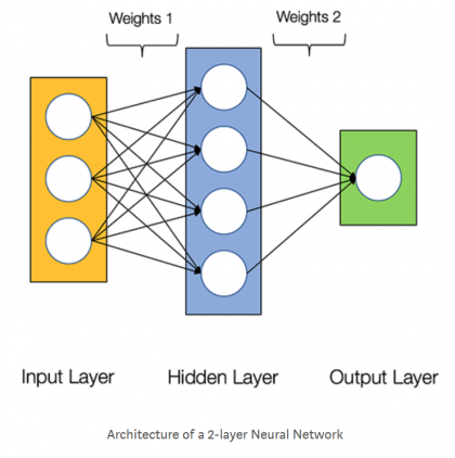
, 10 . , (10, 3). “ ”, . , . , :

, , 0 50 ;

X=np.random.randint(0, 50, (10, 3))

0 1;

X=np.random.rand(10, 3)

$\ mu = 2$ $\ sigma ^ 2 = 16$ . , , $N (\ mu, \ sigma ^ 2)$ ;

X=4*np.random.randn(10, 3) + 2

$\ mu = 0$ $\ sigma = 1$ , .

, (10, 3) $W ^ {(1)}$ , . , , . , , , $W ^ {(1)}$ (3, 4) . , $(10, 3) (3, 4) \ Flèche droite (10, 4)$ . , $X \ cdot W ^ {(1)}$ (10,4) , - - , . . , UNE (m, n) ( , ) $a_ {i, j}$ , FA) , $f (a_ {i, j})$ ; , , $a_ {1,2} \ Flèche droite f (a_ {1,2})$ , . , $W ^ {(2)}$ , (4, 1) . , $(10, 3) (3, 4) (4, 1) \ Flèche droite (10, 1)$ . , $\ hat {Y}$ 10- (samples) . :

$\ hat {Y} = X \ cdot W ^ {(1)} \ cdot W ^ {(2)}, \ quad \ quad \ hat {Y} _ {i, 0} = X_ {i, j} W_ { j, k} ^ {(1)} W_ {k, 0} ^ {(2)}.$

, . (bias).

. : , , , .

X=np.random.randint(0, 50, (10, 3))
w1=2*np.random.rand(3,4)-1 #       -1  +1
w2=2*np.random.rand(4,1)-1
Y=np.dot(np.dot(x,w1),w2) #   
Y.shape # (10, 1)
Y.T.shape # (1, 10)
(np.dot(Y.T,Y)).shape # (1, 1), ,

. -1 +1, “” ( ).

. f_1 “ ”, - .

$\ hat {Y} _ {i, 0} = f_2 (f_1 (X_ {i, j} W_ {j, k} ^ {(1)}) W_ {k, 0} ^ {(2)}),$ $\hat{Y}=f_2(f_1(X \cdot W^{(1)})\cdot W^{(2)}).$

, .

$\triangle=\sum_i(Y_{i,0}-\hat{Y}_{i,0})^2=\sum_i\widetilde{Y}_{i,0}^2=(\widetilde{Y}.T)_{0,i}\widetilde{Y}_{i,0}=(\widetilde{Y}.T)\cdot\widetilde{Y},$

(X,Y) - , $\widetilde{Y}_{i,0}=Y_{i,0}-\hat{Y}_{i,0}$ . , $(\widetilde{Y}.T)_{0,i}=\widetilde{Y}_{i,0}$ .

, . .

. - . , . , .

- , . f(x) $f^{'}(x_0)=0$ , “ ” - . , , . , , . : - , , - . (, 16 ), , . . , $f^{'}(W)<0$ , , , $f^{'}(W)>0$ , . , .

$W\Rightarrow W+\mu\cdot\delta W=W-\mu\cdot\frac{\partial \triangle}{\partial W},$

$W_{i,j}\Rightarrow W_{i,j}+\mu\cdot\delta W_{i,j}=W_{i,j}-\mu\cdot\frac{\partial \triangle}{\partial W_{i,j}},$

$\mu$ - (learning rate). , . . - , , . , - .

.

$\frac{\partial a_{m, n}}{\partial a_{i,j}}=\delta_{m,i}\delta_{n,j},$

$\delta_{i,j}$ - , , i=j . , $\delta_{1,1}=1$ , $\delta_{2,1}=0$ . : .

$\frac{\partial \triangle}{\partial W_{m,n}}=-2\sum_i(Y_{i,0}-\hat{Y}_{i,0})\frac{\partial \hat{Y}_{i,0}}{\partial W_{m,n}}=-2\widetilde{Y}_{i,0}\frac{\partial \hat{Y}_{i,0}}{\partial W_{m,n}},$

, , $\widetilde{Y}_{i,0}=Y_{i,0}-\hat{Y}_{i,0}$ , .

. . , , .

, $\hat{Y}_{i,0}=X_{i,j} W_{j,k}^{(1)} W_{k,0}^{(2)}$ ,

$\frac{\partial \triangle}{\partial W_{m,0}^{(2)}}=-2\widetilde{Y}_{i,0}\frac{\partial \hat{Y}_{i,0}}{\partial W_{m,0}^{(2)}}=-2\widetilde{Y}_{i,0}X_{i,j} W_{j,k}^{(1)}\delta_{k,m}=-2\widetilde{Y}_{i,0}X_{i,j} W_{j,m}^{(1)}=-2\widetilde{Y}_{i,0}(X\cdot W^{(1)})_{i,m}$

, $A_{i,m}=(A.T)_{m.i}$ . , :

$\delta W_{m,0}^{(2)}=-\frac{\partial \triangle}{\partial W_{m,0}^{(2)}}=2((X\cdot W^{(1)}).T)_{m,i}\widetilde{Y}_{i,0},$

$\delta W^{(2)}=2((X\cdot W^{(1)}).T)\cdot \widetilde{Y}.$

, , , $\delta W^{(2)}$ . $X\cdot W^{(1)}$ (10,3)(3,4)=(10,4) , - (4,10) . $\widetilde{Y}$ $\hat{Y}$ - (10,1) . , $\delta W^{(2)}$ (4,10)(10,1)=(4,1) , .

deltaW2=2*np.dot(np.dot(X,w1).T,Y)
deltaW2.shape # (4,1)

$W^{(1)}$ .

$\frac{\partial \triangle}{\partial W_{m,n}^{(1)}}=-2\widetilde{Y}_{i,0}\frac{\partial \hat{Y}_{i,0}}{\partial W_{m,n}^{(1)}}=-2\widetilde{Y}_{i,0}X_{i,j} \delta_{j,m}\delta_{k,n}W_{k,0}^{(2)}=-2\widetilde{Y}_{i,0}X_{i,m} W_{n,0}^{(2)}=-2(X.T)_{m,i}\widetilde{Y}_{i,0}(W^{(2)}.T)_{0,n},$ $\delta W^{(1)}=2(X.T)\cdot \widetilde{Y}\cdot (W^{(2)}.T).$

, “ ”, “ ” - . , , . : “” ( ), , .

$\delta W^{(1)}$ : (3,10)(10,1)(1,4)=(3,4) .

. ,, , , . . , . , . , , : z=f(y(x)) , $z_x^{'}=f_y^{'}y_x^{'}$ .

$\hat{Y}_{i,0}=f_2(f_1(X_{i,j} W_{j,k}^{(1)})W_{k,0}^{(2)})\quad\Rightarrow\quad \hat{Y}_{i,0}=f_2(C_{i,0}),$

$C_{i,0}=B_{i,k}W_{k,0}^{(2)}, \quad\quad B_{i,k}=f_1(A_{i,k}), \quad\quad A_{i,k}=X_{i,j} W_{j,k}^{(1)}.$

W_2 , . ,

$\delta W_{m,0}^{(2)}=2\widetilde{Y}_{i,0}\frac{\partial \hat{Y}_{i,0}}{\partial W_{m,0}^{(2)}}=2\widetilde{Y}_{i,0}\frac{\partial f_2(C_{i,0})}{\partial C_{\mu,0}}\frac{\partial C_{\mu,0}}{\partial W_{m,0}^{(2)}}=2\widetilde{Y}_{i,0}f_2^{'}(C_{i,0})\delta_{i,\mu}B_{\mu,k}\delta_{k,m}=2\widetilde{Y}_{i,0}f_2^{'}(C_{i,0})B_{i,m}.$

$\frac{\partial f_2(C_{i,0})}{\partial C_{\mu,0}}=f_2^{'}(C_{i,0})\delta_{i,\mu}, \quad\quad \frac{\partial C_{\mu,0}}{\partial W_{m,0}^{(2)}}=B_{\mu,k}\frac{\partial W_{k,0}^{(2)}}{\partial W_{m,0}^{(2)}}=B_{\mu,k}\delta_{k,m}.$

, - . : $B_{i,m}=(B.T)_{m,i}$ , $f_1(A_{i,m})=(f_1(A).T)_{m,i}$ . ,

$\delta W_{m,0}^{(2)}=2(B.T)_{m,i}\widetilde{Y}_{i,0}f_2^{'}(C_{i,0}) \Rightarrow \delta W^{(2)}=2(B.T)\cdot(\widetilde{Y}*f_2^{'}(C))$

“*” . , , , a*b , ; , $a_{1,2}b_{1,2}$ .

. f_1(x)=x^2 f_2(x)=x^3 . , , . NumPy .

def f1(x): #  
    return np.power(x,2)
def graf1(x): # 
    return 2*x
def f2(x): #  
    return np.power(x,3)
def gradf2(x): # 
    return 3*np.power(x,2)

A=np.dot(X,w1) #   
B=f1(A)        #   
C=np.dot(B,w2) #    
Y=f2() #   
deltaW2=2*np.dot(B.T, Y*gradf2(C))
deltaW2.shape # (4,1)

$W^{(1)}$ , . - .

$\delta W_{m,n}^{(1)}=2\widetilde{Y}_{i,0}\frac{\partial \hat{Y}_{i,0}}{\partial W_{m,n}^{(1)}}=2\widetilde{Y}_{i,0}\frac{\partial f_2(C_{i,0})}{\partial C_{\mu,\nu}}\frac{\partial C_{\mu,\nu}}{\partial B_{l,s}}\frac{\partial B_{l,s}}{\partial W_{m,n}^{(1)}},$

$C_{\mu,\nu}=B_{\mu,k}W_{k,\nu}^{(2)}$ . :

$\frac{\partial f_2(C_{i,0})}{\partial C_{\mu,\nu}}=f_2^{'}(C_{i,0})\delta_{i,\mu}\delta_{0,\nu},\quad\quad \frac{\partial C_{\mu,\nu}}{\partial B_{l,s}}=\delta_{\mu,l}\delta_{k,s}W_{k,\nu}^{(2)},\quad\quad$ $\frac{\partial B_{l,s}}{\partial W_{m,n}^{(1)}}=\frac{\partial B_{l,s}}{\partial A_{r,e}}\frac{\partial A_{r,e}}{\partial W_{m,n}^{(1)}}=f_1^{'}(A_{l,s})\delta_{l,r}\delta_{s,e}\delta_{j,m}\delta_{e,n}X_{r,j}=f_1^{'}(A_{l,s})\delta_{l,r}\delta_{s,n}X_{r,m}.$

$\ delta W_ {m, n} ^ {(1)} = 2 \ widetilde {Y} _ {i, 0} f_2 ^ {'} (C_ {i, 0}) \ delta_ {i, \ mu} \ delta_ {0, \ nu} \ delta _ {\ mu, l} \ delta_ {k, s} W_ {k, \ nu} ^ {(2)} f_1 ^ {'} (A_ {l, s}) \ delta_ {s, n} \ delta_ {l, r} X_ {r, m} = 2 \ widetilde {Y} _ {i, 0} f_2 ^ {'} (C_ {i, 0}) W_ {n, 0} ^ {(2)} f_1 ^ {'} (A_ {i, n}) X_ {i, m},$

$\ delta_ {i, \ mu} \ delta_ {0, \ nu} \ delta _ {\ mu, l} \ delta_ {k, s} \ delta_ {s, n} \ delta_ {l, r} = \ delta_ { i, l} \ delta_ {i, r} \ delta_ {k, n} \ delta_ {s, n}.$

, $\ delta_ {0, \ nu} W_ {k, \ nu} ^ {(2)} = W_ {k, 0} ^ {(2)}$ , , “”, l, r, k, s .

“” ,

$\ delta W_ {m, n} ^ {(1)} = 2 (XT) _ {m, i} \ widetilde {Y} _ {i, 0} f_2 ^ {'} (C_ {i, 0}) ( W ^ {(2)}. T) _ {0, n} f_1 ^ {'} (A_ {i, n}),$ $\ delta W ^ {(1)} = 2 (XT) \ cdot [[(\ widetilde {Y} * f_2 ^ {'} (C)) \ cdot (W ^ {(2)}. T)] * f_1 ^ {'} (A)].$

, $D_ {i, o} = \ widetilde {Y} _ {i, 0} f_2 ^ {'} (C_ {i, 0}) \ Rightarrow \ widetilde {Y} * f_2 ^ {'} (C)$ , $F_ {i, n} = D_ {io} (W ^ {(2)}. T) _ {0, n}$ , $F_ {i, n} f_1 ^ {'} (A_ {i, n}) \ Flèche droite F * f_1 ^ {'} (A)$ .

deltaW1=2*np.dot(X.T, np.dot(Y*gradf2(C),w2.T)*gradf1(A))
deltaW1.shape # (3,4)

. .

“, - . -!” ? , , , . , . - , , . ! , , - . , , .

, . James Loy - , , , , , . . , , , . “-”, , , . , TensorFlow Keras. , la source originale (il existe une traduction en russe).

Écrivez des codes, fouillez dans des formules, lisez des livres, posez-vous des questions.

Quant aux outils, ce sont Jupyter Notebook ( règles Anaconda !), Colab ...

Matrice-Rematrix

-

!

.

More articles: