🖖 😌 😀 L'art ancien de la nomographie 🧑🏾‍🤝‍🧑🏼 👩🏾‍⚕️ 👸🏾

J'ai vu pour la première fois ce graphique étrange dans un laboratoire universitaire. Un morceau de papier quelconque, photocopié d'un vieux livre, a été collé sur le mur à côté de l' évaporateur rotatif . La feuille, évidemment, a été souvent utilisée, mais elle a été soignée, comme si elle contenait un ancien sortilège puissant ... Par la suite, je suis tombé sur des graphiques similaires dans d'autres laboratoires, comme s'ils faisaient partie intégrante de la distillation avec vide. Ensuite, des dessins similaires ont été trouvés sur les pages de diverses littératures techniques. On les appelait nomogrammes . Il s'est avéré ridiculement facile d'apprendre à les utiliser, mais qui et comment les a fabriqués à un moment donné est resté un mystère.

À quoi ressemblent les nomogrammes et comment ils fonctionnent

Un nomogramme qui est souvent utilisé dans la distillation sous vide est illustré dans la figure ci-dessous.

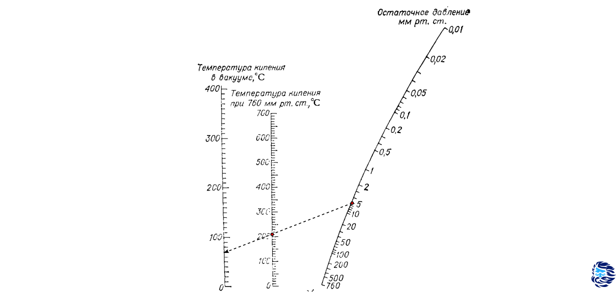
, , (), . , , , — , . , . 760 100 , , 40 34 .

-, 204 ? " 760 " 204 , " " 5 , . , , 70 .

. . , . , $y=f(x)$ ?

— . , , . — , — .

(1884—1891) — «». Traité de nomographie. Théorie des abaques. Applications pratiques . . , — The Lost Art of Nomography by Ron Doerfler.

, !

: . , — :

\frac{d \ln p}{d T} = \frac{Δ H_{v a p}}{R T^{2}}

$\frac{d \ln p}{dT} = \frac{\Delta H_{vap}}{RT^2}$

$\Delta H_{vap}$ — , $R$ — .

\ln \frac{p}{p^{*}} = - \frac{Δ H_{v a p}}{R} (\frac{1}{T} - \frac{1}{T^{*}})

$\ln \frac{p}{p^*}=-\frac{\Delta H_{vap}}{R}\left( \frac{1}{T}-\frac{1}{T^*}\right)$

$p^{*}$ 760 , $T^{*}$ — . $T$ $p$ .

Δ S_{v a p} = \frac{Δ H_{v a p}}{T} \approx 10.5 R

$\Delta S_{vap} = \frac{\Delta H_{vap}}{T} \approx 10.5R$

, :

\ln \frac{p}{p^{*}} = 10.5 (1 - \frac{T}{T^{*}})

$\ln \frac{p}{p^*} = 10.5\left(1-\frac{T}{T^*}\right)$

pynomo

— - pynomo. :

pip install pynomo

2 :

F_{1} (u_{1}) = F_{2} (u_{2}) \times F_{3} (u_{3})

$F_1(u_1)=F_2(u_2)\times F_3(u_3)$

$F_i(u_i)$ — - . .

, (RPM) . :

a = ω^{2} \times r

$a = \omega^2 \times r$

#!/usr/bin/env python3
# -*- coding: utf-8 -*-
"""
    rpm.py

    Simple nomogram of type 2: F1=F2*F3
"""
import sys
sys.path.insert(0, "..")
from pynomo.nomographer import *

N_params_RCF={
        'u_min':1000.0,
        'u_max':30000.0,
        'function':lambda u:u,
        'title':r'RCF, $\times g$',
        'tick_levels':3,
        'tick_text_levels':1,
        'tick_side': 'left',
        'scale_type':'linear smart',
        'text_format': r"$%2.0f$",
                }

N_params_r = {'u_min': 1.0,
              'u_max': 5.0,
              'function': lambda u:u,
              'tick_levels': 3,
              'tick_text_levels': 1,
              'tick_side': 'left',
              'text_format': r"$%2.0f$",
              'title':r'R, cm',
              'extra_params': [
                {'u_min':  5.0,
                 'u_max': 10.0,                 
                 'tick_levels': 2,
                 'tick_text_levels': 1,
                 'tick_side': 'right',
                 'text_format': r"$%2.0f$",},
                {'u_min': 10.0,
                 'u_max': 40.0,
                 'scale_type': 'manual line',
                 'manual_axis_data': {10.0: r'10',
                                      12.0: r'12',
                                      14.0: r'14',
                                      16.0: r'16',
                                      20.0: r'20',
                                      24.0: r'24',
                                      30.0: r'30',
                                      40.0: r'40'},
                 },
                ],
            }

N_params_RPM={
        'u_min': 1000.0,
        'u_max':20000.0,
        'function':lambda u:u*u*1.1182e-5,
        'title':r'RPM',
        'tick_levels':3,
        'tick_text_levels':1,
        'scale_type':'linear smart',
        'text_format': r"$%2.0f$",
                }

block_1_params={
             'block_type':'type_2',
             'mirror_y':True,
             'width':10.0,
             'height':10.0,
             'f1_params':N_params_RCF,
             'f2_params':N_params_r,
             'f3_params':N_params_RPM,
             'isopleth_values':[['x',10.0,15200]],
             }

main_params={
              'filename':'RPM.pdf',
              'paper_height':10.0,
              'paper_width':10.0,
              'block_params':[block_1_params],
              'transformations':[('rotate',0.01),('scale paper',)],
              'title_str':r'$a=r\times \omega^2$'
              }
Nomographer(main_params)

$F_3(u_3) = \omega^2$ :

'function':lambda u:u*u*1.1182e-5,

RPM.pdf, .

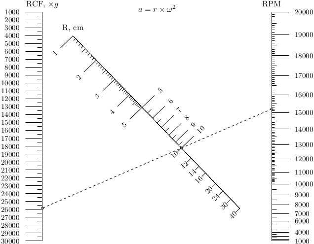
— , ( g) ( ) (RPM).

? .

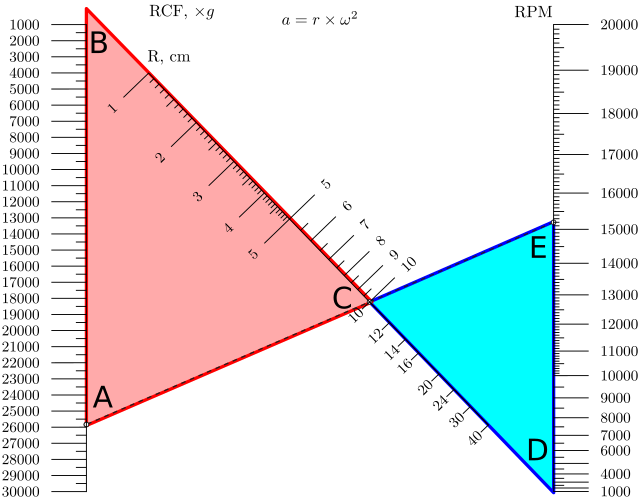
, ABC CDE — . :

\frac{A B}{E D} = \frac{B C}{C D} = \frac{B C}{L - B C}

$\frac{AB}{ED} = \frac{BC}{CD} = \frac{BC}{L-BC}$

L — BD, . , L.

\ln \frac{p}{p^{*}} + 10.5 = \frac{10.5 T}{T^{*}}

$\ln \frac{p}{p^*}+10.5=\frac{10.5T}{T^*}$

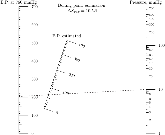
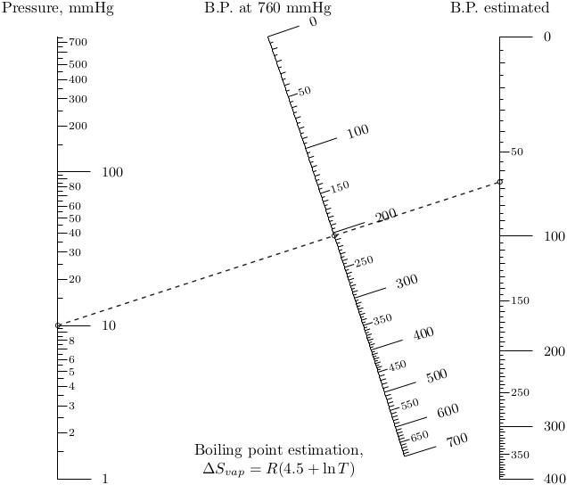
, , . Trouton–Hildebrand–Everett:

\frac{Δ H_{v a p}}{R T} = (4.5 + \ln T)

$\frac{\Delta H_{vap}}{RT} = (4.5 + \ln T)$

Some calculations for organic chemists: boiling point variation, Boltzmann factors and the Eyring equation. Tetrahedron Letters 41 (2000) 9879–9882 , . !

\ln \frac{p}{p^{*}} + T^{*} (4.5 + \ln T^{*}) \times \frac{1}{T} - (4.5 + \ln T^{*}) = 0

$\ln \frac{p}{p^*} + T^{*}(4.5 + \ln T^*)\times \frac{1}{T}-(4.5 + \ln T^*) =0$

F_{1} (u) + F_{2} (v) F_{3} (w) + F_{4} (w) = 0.

$F_1(u)+F_2(v)F_3(w)+F_4(w)=0.$

. .

from math import log
from pynomo.nomographer import *
import sys
sys.path.insert(0, "..")

Pressure = {
    'u_min':  1.0,
    'u_max': 760.0,
    'function': lambda u: log(u / 760.0),
    'title_y_shift': 0.55,
    'title': r'Pressure, mmHg',
    'tick_levels': 3,
    'tick_text_levels': 2,
    'scale_type': 'log smart',
}

BP_guess = {
    'u_min':  0.0,
    'u_max': 400.0,
    'function': lambda u: 1/(u + 273.15),
    'title_y_shift': 0.55,
    'title': r'B.P. estimated',
    'tick_levels': 4,
    'tick_text_levels': 2,
    'scale_type': 'linear smart',
}

BP_at_atm = {
    'u_min':  0.0,
    'u_max': 700.0,
    'function_3': lambda u: (u + 273.15)*(4.5 + log(u + 273.15)),
    'function_4': lambda u: -(4.5 + log(u + 273.15)),
    'title_y_shift': 0.55,
    'title': r'B.P. at 760 mmHg',
    'tick_levels': 4,
    'tick_text_levels': 2,
    'scale_type': 'linear smart',
}

block_1_params = {
    'block_type': 'type_10',
    'width': 10.0,
    'height': 10.0,
    'f1_params': Pressure,
    'f2_params': BP_guess,
    'f3_params': BP_at_atm,
    'isopleth_values': [[10, 'x', 204]]
}

main_params = {
    'filename': 'ex_type10_nomo_1.pdf',
    'paper_height': 10.0,
    'paper_width': 10.0,
    'block_params': [block_1_params],
    'transformations': [('rotate', 0.01), ('scale paper',)],
    'title_y': 0.55,
    'title_str': r'Boiling point estimation, $\Delta S_{vap} = R(4.5 + \ln T)$'
}

Nomographer(main_params)

, . , — , . , , . .

10% !

L'art ancien de la nomographie

À quoi ressemblent les nomogrammes et comment ils fonctionnent

pynomo

More articles: